Category: Uncategorized

This week was spring break

One of our tasks last week was to make a diagram that provides an overview of our project’s methods, pictured below. The blue represents inputs, the yellow represents a function (our semi-supervised method), the green represents outputs, and the purple is the final output.

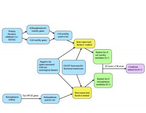
At the top of the diagram, the blue boxes go through the process of creating the positive list of cell motility genes. The genes were gathered from different signaling pathways in the KEGG database as well as studying primary literature. From these resources, I created two separate positive lists: one purely of cell motility genes and one of cell motility genes implicated in schizophrenia. I combined these together (collapsing the duplicates) in order to create a positive list of 541 cell motility genes. At the bottom of the diagram, the two blue boxes go through the process of creating the schizophrenia positive list. Alex pulled schizophrenia genes from genome-wide association studies (GWAS), then filtered the genes down to the top 300 positives by taking into account their p-values from the literature. We each ran the semi-supervised iterative method on the GIANT brain interactome with the same negative set, differing only in the positive sets we used. From there, the iterative method spit out ranked lists of schizophrenia candidates and cell motility candidates with scores ranging from 0-1 (the green boxes.) Finally, we combined the scores by multiplying them to take into account their probability of being “good” candidates for both cell motility and schizophrenia (the purple box.)

The CREU diagram can also be viewed here.

Our runtime-shortening strategies seemed to have worked well! We plotted runtime vs. iteration number and found that each iteration took about 3-4 seconds, so there’s no increase as we saw last time. However, we did find that the scores do not change after a surprisingly small number of iterations, so we will be tweaking a few things to see what changes.

Because it’s hard to tell if a semi-supervised machine learning method is actually good at what it’s supposed to accomplish, we will also be looking into ways to test our method.

Our goals for next time include:

1. Run on a larger portion of the network. So far we have been using the 0.200 probability threshold network, but we will move down to 0.150 threshold.
2. Change the number of positives used – see what the effect is of using 1 vs. 300+ positives on the graph.
3. Plot a distribution of the ranked candidate scores.
4. Plot the absolute value of the sum of changes made during each iteration.
5. Look into cross validation to check if our method is doing a good job at what it’s supposed to do. This involves hiding some positives from your positive list and seeing if your method correctly identifies these hidden positives as having a high probability (if not the highest) of being involved in the pathway.
6. Look  into how other papers were able to be convincing about the accuracy of their method.

Next week is spring break so there will be no blog post!

 

Last week we had the task of running our algorithm for 100,000 iterations. We ran into a couple of problems:

1. It took a very long time. We actually stopped running it at about 1300 iterations (which took 12 hours) because the estimated time kept increasing. There are a few lines in our code that we are going to change to improve running time – we will convert some variables we’re using to track changes between iterations from lists of nodes to integer counts.
2. The difference in score we wanted to see before stopping iterations was far too big. We allowed the code to run until the difference in scores between iterations was no more than 0.001 (or it hit 100,000 iterations), and to our surprise, it took around 130 and 180 iterations for cell motility and schizophrenia positives, respectively. Because the scores range from 0 to 1, a change of 10^-4 is bigger than we initially thought. After speeding up the code, we are going to run it until we see changes less than 10^-9.

We are also going to create a histogram of run time versus progress (each iteration) to track our algorithm and see if there is a separate problem that causes the code to slow down as the number of iterations increases.

Our continued goals for this week are to BLAST candidates to see if they are conserved in Drosophila. 

We needed to find drosophila analogs to the genes high on our list, so this week, we built a program that converts human gene names to human protein ID numbers from the NCBI. Then, the ID number is put into BLAST, a tool from the NCBI that sorts drosophila proteins by amino residue sequence similarity.

There are also things we can do to optimize the gene ranker program to improve the run time. We will be converting some sets to integers and will catalog the runtime versus the progress.

Anna noted that we need to run the program for quite a bit longer to get a more accurate result, so we’ll publish those results in a couple of days.

Also, we need to find out if our candidate genes are conserved in drosophila. We can use this with BLAST, an NCBI tool that lets us compare sequence similarity across species. Rather than do it manually, we’ll hook it up directly to our terminal.

We have two goals to accomplish for our meeting next week:

1. Run our iterative method for 100,000 iterations, or until the scores change by 0.001 or less. See how this affects the ranking compared to 150 iterations. Will it just affect the scores but not the relative rankings?
2. See if the candidates are conserved in drosophila melanogaster. The second part of this project is to experimentally validate the candidates, which we cannot do if they aren’t conserved in drosophila. As a quick sanity check, we’re going to BLAST CTNNB1 (the well-studied Catenin Beta 1 gene that codes for a protein involved in the formation of adherens junctions) in humans against drosophila which should be ARM.

The results will be posted in a couple of days.

This previous week we put our iterative algorithm to the test. Alex and I each ran our positive (and negative) lists for 150 iterations using the 0.200 threshold GIANT brain network. As a reminder, the 0.200 threshold network is a trimmed version of the GIANT network where all the edges have probability scores of 0.200 or greater.

I used all 541 of my positives, a combination of two sublists: cell motility genes and cell motility genes implicated in schizophrenia. In the upcoming weeks, I will experiment with running these two lists separately and seeing how the results are affected.

I also used Alex’s list of negatives, which are genes expressed in other organs but not the brain. We will need to closely consider whether it is wise to use this set of negatives alongside cell motility positives.

Even with these two potential issues, our preliminary lists of candidates looked promising – for example, one gene we found is Hes Related Family BHLH Transcription Factor With YRPW Motif 2, also know as HEY2. HEY2 was not only a schizophrenia positive but was also moderately high in the list of cell motility candidates, with a score of 0.56. Another gene we uncovered was 1-Acylglycerol-3-Phosphate O-Acyltransferase 4, or AGPAT4. This was not in either list of positives, but it was given the maximum score of 1.0 in each set of candidates. Both of these genes point to the different ways we can analyze our results and what it means to be a promising candidate – do we care about genes that are positives in the schizophrenia set and are determined by the algorithm to likely be involved in cell motility or do we care about genes that are determined by the algorithm to be likely involved in cell motility and schizophrenia? Do we care about both? What is the difference? Is one more promising than the other?  In the upcoming weeks, we will be figuring out these questions in order to refine our list of candidates.

We will also be extending the time that our algorithm runs. 150 iterations may seem like a lot, but cutting the algorithm short may lead to “stunted” results. The iterative method can be thought of as dyes from the positive and negative nodes spreading throughout the network, staining the surrounding nodes in a way that reflects their distances from the positives and negatives. If the iterations are stopped before they converge (i.e. subsequent iterations don’t change the scores, or color of the node), then the color of the nodes might be closer to the color of the positives and negatives than they should be. Our next step will be to let it run for 1500 iterations and see how our results our affected.

Out of my own curiosity, I also decided to see if all of the cell motility positives were in the GIANT network, which turned out to be false. There are about 40 genes (out of 541) that are not in the GIANT network. However, I don’t believe this to be a problem; if there are positive cell motility genes not in the GIANT network, it is probably because not all genes involved in cell motility are expressed in every type of cell and are therefore not relevant in a brain-specific network.

It works! Our program made a list of candidate genes. After 150 iterations, the SZ positives made a novel list of genes that may be involved in Schizophrenia, ranging from potassium gating to Golgi associated proteins to proteins involved in cellular motility. This program can be refined, and so we will spend the upcoming weeks narrowing the list and making sure that this process can be as precise and accurate as it can be.

Another thing that I did myself was rank SZ genes, since I didn’t want to include all 2700 genes that are implicated. First, for every dataset (Psychiatric Genomics Consortium, Common Mind Consortium, SZGene, hiPSC rtRNA results, chromosome conformation predictions), I gathered the magnitude of the change in expression/ the frequency of mutation  and the p value for each gene. Then I took the log base 2 of the change and the negative log base 2 of the p value and multiplied them together.

There are a couple of important things to note. Schizophrenia is primarily a regulation problem. As the Psychiatric Genomics Consortium study pointed out, there is very little genetic variation in SZ patients from control patients in coding regions; there are only a dozen significant mutations in coding regions. Of all the mutations, the one with the highest confidence, with a p value of 10^-15, has a frequency in SZ patients at 0.87 and a frequency in control patients at 0.85. SZ is undeniably a confluence of many, possibly hundreds or thousands, of tiny genetic variations.

Apparently, many of these mutations are common among several major psychiatric disorders. An article was recently published in Science that showed that Schizophrenia, Bipolar Disorder, Depression, and Autism all have highly correlated patterns of cortical gene expression (http://science.sciencemag.org/content/359/6376/693.full). The tool we are developing will hopefully be powerful enough to help us identify the underlying causes of these diseases.

We have a couple of goals for next week: fix a subtle yet major bug in our iterative method program and then run it on our gene lists to get a preliminary list of candidate genes. I will also write a short program to compare the genes in the GIANT network to the list of cell motility genes.

We got our program built! It works with the tiny network example that we gave it, with a couple of bugs, which we will fix this week. Also by next week, we will have a preliminary list of candidate genes.