About 3D Modeling and Printing


Perhaps you’re interested in 3D printing? Though full of possibilities, 3D printing has remained outside the realm of casual tinkering because of cost, accessibility, and standard procedure. Recently however, 3D printing has become relatively cost-friendly! You don’t even have to own your own printer; companies such as shapeways will print your models for you at a (usually) reasonable cost! Many universities are adopting one or more 3D printers as well (even non-engineering-or-design schools, such as Reed), so if you are student there is a good chance that you can get access to a printer in person. If you are intrigued by the actual printing process yourself, this is a great blog for technical info: Reed College Fab Lab. Continue reading “About 3D Modeling and Printing”
Visualizing Green’s Theorem

If you are or have been a student of mathematics, physics, or engineering, you have likely encountered the following equation:

$$\oint_C Pdx + Qdy = \iint_D \left ( \frac{\partial Q}{\partial x} – \frac{\partial P }{\partial y} \right )dA$$

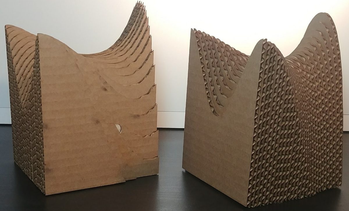
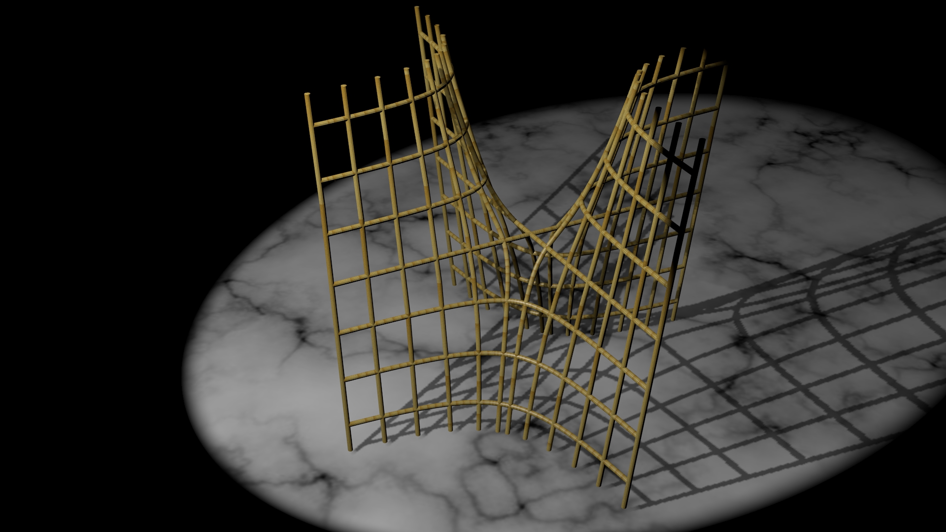
This statement, known as Green’s theorem, combines several ideas studied in multi-variable calculus and gives a relationship between curves in the plane and the regions they surround, when embedded in a vector field. While most students are capable of computing these expressions, far fewer have any kind of visual or visceral understanding. In this post, I want to build some of that understanding by discussing each component of the theorem in a visual way. My hope is that, armed with the right intuitions, Green’s theorem should feel nearly natural.
Continue reading “Visualizing Green’s Theorem”

Iterated Integrals

What is a multiple integral? The notion itself is fairly intuitive: we stretch the notion from single variable calculus of “the area under a function’s graph” to higher dimensions, resulting in the multidimensional analogue of area, volume (or hypervolume). A multiple integral is essentially a way of quantifying the spatial “footprint” that a region or the graph of a function has. It is computable by splitting the region into many smaller pieces, but there is some art to performing this dissection.

Continue reading “Iterated Integrals”

Level Sets, the Gradient, and Gradient Flow

Level sets, the gradient, and gradient flow are methods of extracting specific features of a surface. You’ve heard of level sets and the gradient in vector calculus class – level sets show slices of a surface and the gradient shows a sort of 2D “slope” of a surface. These measurements are useful on their own, but they hint at something else, something more abstract. The gradient vectors are perpendicular to the level sets, so will always be direction the “slope” of a point toward another point on another level set. But how would you represent that? The answer is the concept of gradient flow. Read more to learn about how these three standard measurements fit together to flow along a surface, much like a liquid or rolling object.
Continue reading “Level Sets, the Gradient, and Gradient Flow”

Visualizing multivariable functions and their derivative

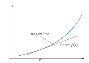
In a first course in calculus, many students encounter an image similar to the following:


Such an illustration highlights a key property of the single variable derivative: it’s the best linear approximation of a function at a point. For functions of more than one variable, the derivative exhibits this same characteristic, yet there is no obvious corresponding picture. What would an analogous visualization look like for a multivariable function?

For the past few weeks, I’ve been working towards a visualization of multivariable functions and their derivatives. Check out the end result here, or read on to hear about my process. I assume some knowledge of calculus and mathematical notation.

Continue reading “Visualizing multivariable functions and their derivative”