
Hi! I’m Lixing Yi, a rising sophomore, and this summer I have been implementing code to count directed graphlets and utilizing the data to categorize biological networks. Intending to be a math major, I have spent more of my time on the theoretical aspect of things. While I’ve learned about graphs and algorithms before, working on this project has been a refresher, as it’s a different way of interaction with these math concepts- to think about what the results means in a real-world context; to do a lot of trials and errors instead of “pure thinking”. It’s also an eye-opener for me to realize the vast opportunities in fields that I’ve not thought of before.
What are directed graphlets?
Graphlets are small, connected simple graphs. In our context, a graphlet is usually not alone an entire graph but an induced subgraph of a bigger graph. And namely, directed graphlets are graphlets with directed edges, like arrows between two nodes (vertices). For our context, we also allow bi-directional edges, which are edges that has arrows on both ends and can go both ways. We represent those edges by a pair of opposite-pointing edges.
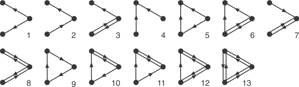
Now we can define orbits. Node orbit are labels assigned to node positions in a graphlet. Intuitively, two nodes have the same orbit if they are symmetric. Rigorously, it means that permuting the two nodes with the same orbit will result in the exact same graphlet. Edge orbit follows the same idea, and it can be determined by node orbits: two edge have the same edge orbit if and only if the node orbits on their end nodes are the same.
That’s a brief introduction of graphlets! Hannah also explains the undirected version in her post. We are interested in them because the occurrence (or the lack of) these small graphs as induced subgraphs of a bigger graph might suggest interesting information of the big graph. On a node-level, the orbits that a node participates in can say things about the functionality of that node. Many biological networks are directed graphs, but due to the complexity of directed graphlets, our earlier work treats the edges as undirected. Thus, my work focuses on making tools to enable analysis with directed graphlets.
How do we count them?
Before discussing all the tricks to make the counting faster, let’s see the bottom line: There is always the brute force method. If we want to count all the four-node graphlets for example, we need to exhaust every connected four-node groups, and match this group with one of all 199 four-node graphlets. In comparison, there are only 6 undirected four-node graphlets. Each matching test is a mini graph isomorphism problem, so the run time adds up quickly, making the brute force method unideal.
To make the search more efficient, we use a method named GTrie, developed by Pedro Rebeiro et al. In short, it uses a decision tree to reduce the search space of graphlets we try to match. At every node, we start a BFS search to find all graphlets involved with it. Every time we discover a new node, we gain partial information about the potential graphlets and can eliminate some choices. For example, If the algorithm discovers a bi-directed edge during the search, then it will skip all graphlets without bi-directed edges at the final matching step. If it discover a triangle, then it will get rid of graphlets containing no triangles. When a graphlet is matched, the algorithm updates the graphlet and orbit counts. For a more detailed introduction, please refer to Rebeiro’s paper.
Another general approach to count directed graphlets is to count only certain graphlets, and then combinatorially build linear equations and compute the counts for the rest based on this information. This method is indeed faster than the Gtrie approach and is the one we use for undirected graphlet analysis. However, due to the complexity of directed graphlets, building linear equations becomes much more difficult and time-consuming that it outweighs the run time advantage. Another practical factor is that Gtrie already has code implementation while the linear equation approach only has a theoretical description. Behind the scenes, most of my time has been spent on configuring the Gtrie implementation to work.
Why do we count them?
Directed graphlet and orbit counting has many applications, but for our project we mainly used graphlet counting to characterize different biological networks. Beyond the number of nodes and edges, graphlet count provides substantially more dimensions for network comparison. In simple terms, we are now able to say “network A is different than network B in the sense that A has much fewer graphlet no. 5, but they both have similar number of graphlet no. 27.” However, we can’t just naively compare the graphlet counts of two networks directly, as the two networks might have very different sizes and inherently have very different graphlet counts. A direction of improvement would be to normalize the graphlet count by the number of nodes and edges. But how exactly? Since graphlets are very different than nodes or edges, we can’t just divide the grpahlet count by node count or edge count. For this task, we chose the Erdős–Rényi model, a random graph generating model. Given the count of a specific graphlet in a specific network, we calculate the probability1 and the confidence level that this count occurs in an Erdős–Rényi random graph with the same number of nodes and edges2.
Although Erdős–Rényi model serves as a functioning null model for statistical comparison, it might still be “too random” and the confidence level based on this model might not reflect the real-world statistical significance. In a biological context, the more relevant question might be “how does this network compare to networks of similar type?” Clearly, that’s not an easy question. But to at least partially answer the question, we tentatively define “networks of similar type” as networks that have the same degree sequence. In our directed graph context, the notion of degree sequence is trickier with different types of edges, as discussed below3. To generate null-models under this restriction, we used the random-rewire algorithm. It randomly picks two edges (the stricter version would require them to be the same type), swaps the nodes on the edges, and repeats this process many times. This way, it randomizes the network while keeping the degree sequence the same, thus accomplishing our task of generating “networks of similar type”. We then generated 100 such graphs for a given specific network and computed the statistical significance of the graphlet counts for this network comparing to our null model. An example of our results is shown below.
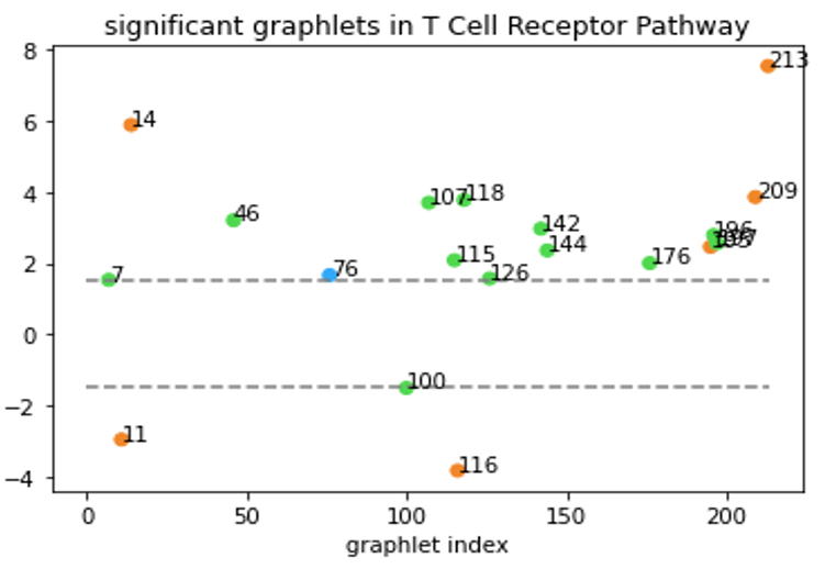
All-bidirectional graphlets are orange, all-one-directional are blue.
Graphlets with both bidirectional and one-directional edges are green.
Now, we are able to say “T Cell Receptor Pathway has a lot of graphlet no. 213” without causing any confusions!
Future work
You might have noticed that I didn’t mention orbits in my work. For the time being, I only get to work on the general graphlet count, but I’m excited to see what new insights we will gain by incorporating node/edge orbits into the analysis. What’s more, we will also incorporate directed graphlet counting with Hannah’s project on MCL clustering for community detection. Some of the networks that Hannah worked on are directed networks, and we are hoping a directed clustering algorithm will bring more accurate results. The clustering algorithm will also require an edge orbit count which the Gtrie software doesn’t do yet, but it’s a fun challenge to devise an algorithm for this task.
Reference
[1] Pedro Ribeiro, Fernando Silva. G-Tries: an efficient data structure for discovering network motifs. https://www.dcc.fc.up.pt/~pribeiro/pubs/pdf/ribeiro-acmsac2010.pdf
[2] The Gtrie implementation that I modified: https://www.dcc.fc.up.pt/got-wave/
Thanks for reading all the way to the end! Here’s the footnotes.
- The probability of an induced subgraph in a Erdős–Rényi graph is discussed here. It’s one of those things that everyone agrees it’s true but no one bothers to give a rigorous proof. (laugh)
- Erdős–Rényi graph generation with a specified edge count: I came up with this algorithm using random shuffle: for a n node graph, create all n2 edges, then do a Fisher-Yates random shuffle. Then just chop off the first k edges, k being the number of edges specified. This algorithm takes O(n2) time, which I don’t think can be further improved.
- In my implementation, only the total degree sequence was kept the same, the in-degree, out-degree, and bi-degree sequence were randomized. Whether this would make sense in our biological context, I’m honestly not sure. The more conservative and strict rule would be to keep the degree sequence of each type of edges the same. But then, I worry such restrictions would be too strict that the randomization won’t accomplish much. For the best results, we would do both methods and see how the results differ.