My name is Tommy Yoon (he/him) and I’m a class of 2024 BMB major. This summer I had the opportunity to continue the work of Max and Henry in finding manganese homeostasis proteins in a collaboration with Shivani Ahuja. This summer, instead of working on a multi-species network for manganese and zinc homeostasis, we decided to focus the question on manganese homeostasis in Bacillus subtilis, a gram-positive model bacteria. We used motif finding, transcriptomic analysis, and a protein-protein interaction network to find other proteins involved in manganese homeostasis, and to find links to other systems which sense manganese or other ions.
Manganese Homeostasis
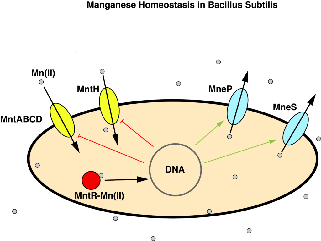
B. subtilis maintains manganese homeostasis with a manganese sensor MntR, which regulates the transcription of uptake proteins MntABCD and MntH, and efflux proteins MneP and MneS.
Motif Finding
We started by looking for the binding motif of MntR in promoter regions of the B. subtilis genome. The idea was that genes with the binding motif would probably be regulated by MntR. We implemented several iterations of a motif finder, including one that looked for clusters of motifs, since MntR often binds in clusters. However, since the information content of the motif is so low, multiple occurrences of the motif showed up before pretty much every gene. It was clear that there are other factors influencing MntR binding, so we moved on to other methods.
Transcriptomics
John Helmann from Cornell graciously supplied some gene expression data from wild-type and mutant mntR samples in both low (50 nM) and high (2.5 µm) concentrations of manganese. By analyzing this data, we can find genes that respond to the absence of mntR and manganese concentration. We looked for genes which responded to a combination of those two factors. Surprisingly, we found a lot of iron uptake genes in this analysis upregulated by a combination of high Mn(II) and mntR mutation. We already knew that high Mn(II) leads to increased expression of iron genes, but this analysis may implicate mntR in the regulation of iron homeostasis.
Network Analysis
We used the STRING protein-protein interaction network to find genes that may be involved in manganese homeostasis. To do this, we used two algorithms: random walk with restarts (RWR) and Omics Integrator. The principle behind these algorithms is that proteins involved in the same process tend to interact with each other more often. If we find out which proteins are interacting with known manganese homeostasis proteins, we may find some candidate proteins that contribute to manganese homeostasis.
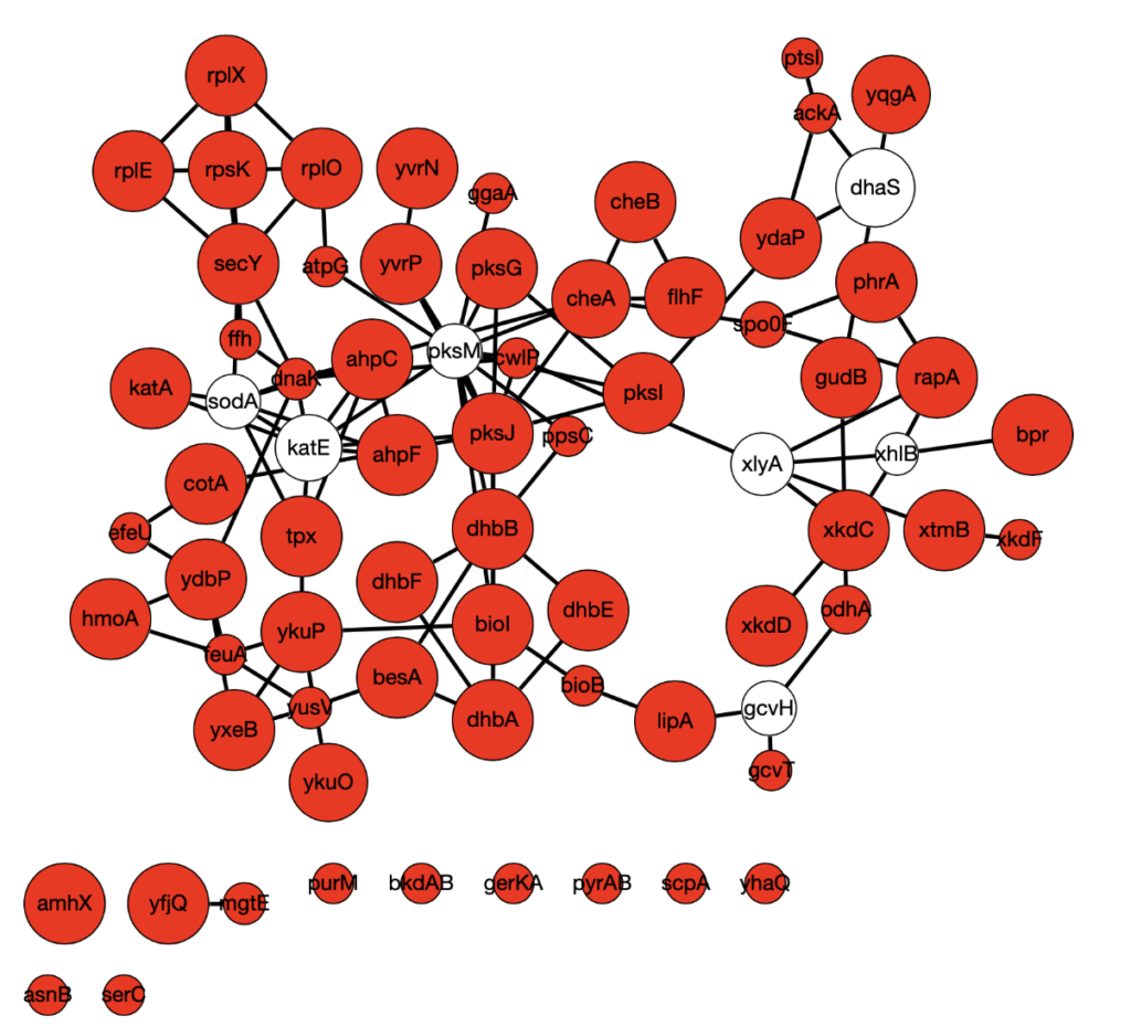
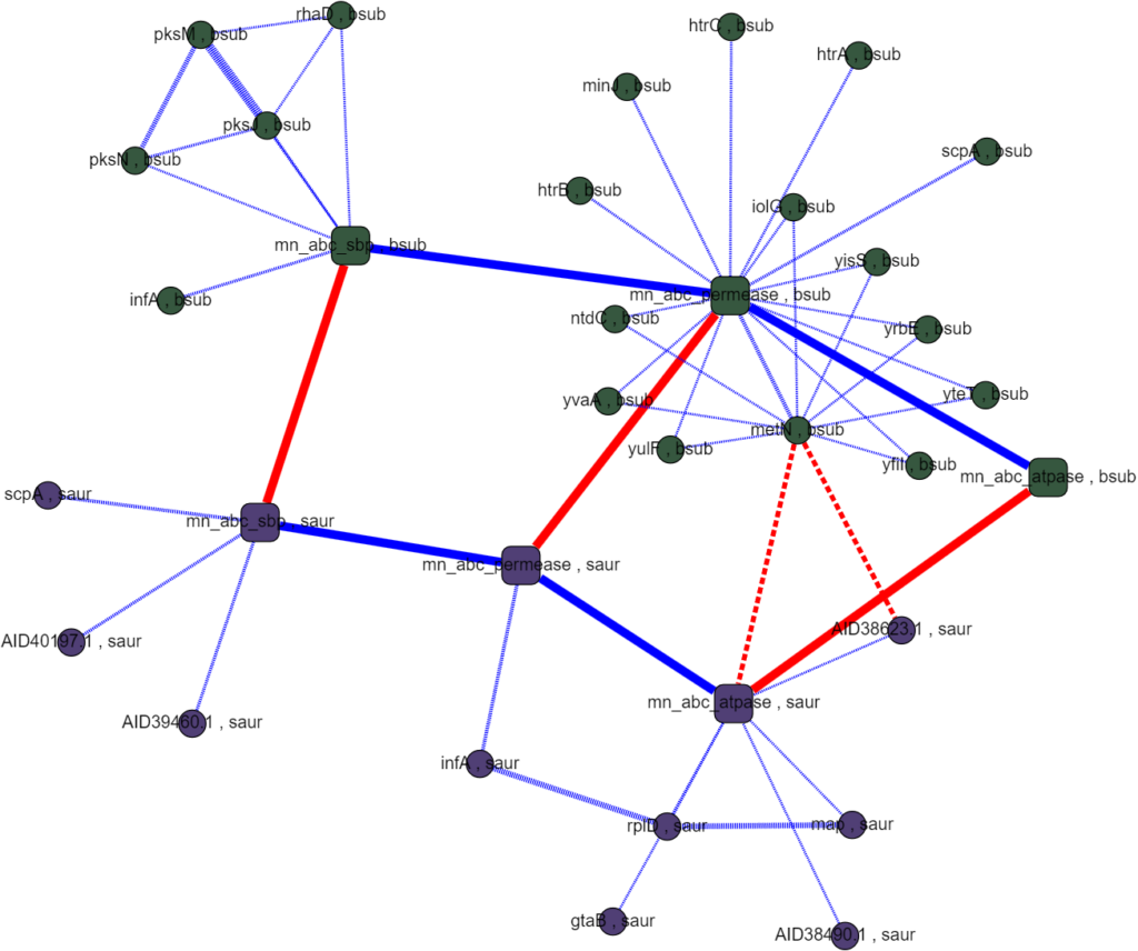
RWR works as follows: start with a source node and walk randomly to connected nodes, keeping track of which nodes are visited. At each step, restart with some probability at another source node. The nodes that get visited the most are strongly connected to the source nodes. Omics Integrator has a similar goal to find nodes that connect your source nodes. Since the known manganese proteins are not very well-connected, we used the differentially expressed genes as our set of source nodes for both of these algorithms. This analysis found a number of central proteins. One surprising find was a magnesium transport protein YfjQ. It is known that magnesium levels are increased in mntR mutants, and so the implication of the magnesium transporter YfjQ in manganese response systems is an interesting result!
Below is a sample Omics Integrator output using downregulated genes as source nodes. Red indicates source nodes and node size indicates how many times the node was found over 900 replicates with different algorithm parameters and source node sets.
There is more computational work to be done here to narrow down on a list of candidates, and more data is always being generated. The door is also open at this point for wet lab work to investigate some of the genes identified in our screen. This is a fun project—I learned a lot about a lot of different things and I’m immensely grateful for the opportunity to work on this project. Big thanks to Anna and the rest of the lab for a great summer!
Hey there, fellow enthusiasts of computer science and molecular intricacies! My name is Ella Ngo (she/her), and I’m a senior pursuing a degree in Computer Science at Reed College. This past summer, I had the incredible opportunity to dive into the world of bioinformatics and contribute to the Signaling Pathway Reconstruction Analysis Streamliner (SPRAS), a powerful tool spearheaded by Anna Ritz, Tony Gitter, and other people at UW-Madison.
Before we embark on this journey, let me provide you with a quick rundown of what Signaling Pathway Reconstruction entails. In a nutshell, it’s about constructing networks composed of different proteins and connecting them based on their known interactions. This approach enables us to uncover pivotal proteins that hold biological significance and warrant further investigation. What makes SPRAS truly remarkable is its ability to consolidate a suite of diverse algorithms, catering to various network analysis methodologies. This democratizes the power of advanced algorithms, making them accessible to users with varying programming backgrounds.
My summer project revolved around understanding the intricate workings of SPRAS and implementing a brand-new algorithm into its framework. Newcomers, including myself, to the SPRAS project embark on an enlightening introductory tutorial, during which we tackle the implementation of a straightforward algorithm called LocalNeighborhood. This process familiarizes us with the program’s structure. Python is the primary language of SPRAS, complemented by SnakeMake and Docker for parallel processing and organized file management, respectively. In the initial phase, I contributed to refining the tutorial, ensuring clarity for future contributors.
After laying a solid foundation through the tutorial, it was time to roll up my sleeves and take on the implementation of the BowTie Builder algorithm – the star of the show. You might wonder what this algorithm does. Well, it’s all about creating a network structure resembling a bowtie. This structure not only highlights crucial regulators and core components but also showcases the downstream elements they influence. Think of it as a molecular flowchart, illustrating the intricate network of proteins in a signaling pathway. BowTie Builder’s magic lies in its ability to uncover intermediate proteins where multiple pathways converge. This valuable insight can uncover potential drug targets, biomarkers, and deeper biological understanding. My task was to integrate BowTie Builder seamlessly into SPRAS, ensuring its compatibility and efficiency. It’s a fascinating algorithm with wide-ranging implications in molecular research and drug development.
Reflecting on the summer, I find myself in awe of Anna Ritz and her team’s dedication to democratizing pathway analysis. By making advanced algorithms accessible and user-friendly, they’re fostering a new era of collaborative research. The work I contributed this summer was like adding a brick to the foundation of SPRAS, strengthening its structure for future innovations and expansions.
As my summer journey with SPRAS comes to an end, I’m filled with gratitude for the opportunity to bridge the worlds of computer science and biology. Anna’s vision and the collective effort of the team inspire me to envision a future where technology propels us closer to unlocking the mysteries of cellular communication. And who knows, maybe the insights derived from SPRAS could revolutionize medicine and beyond.
Until next time, there lies the symphony of life waiting to be decoded. Stay curious, stay passionate, and keep exploring the fascinating realms of science and technology!
Modelling MntABC and ZnuABC Transporter Regulation with Protein Interaction Data from the STRING Database
Hello reader! My name is Max Bennett, I’m a Senior Neuroscience major at Reed College and I’ve spent the summer of 2022 in Anna Ritz’s CompBio lab implementing a protein interactome model to learn more about bacterial metal ion transporters. This work was a collaborative effort with Biochemistry Professor Shivani Ahuja and Junior Biochemistry major Henry Jacques.
Metal Ion Transporters MntABC and ZnuABC
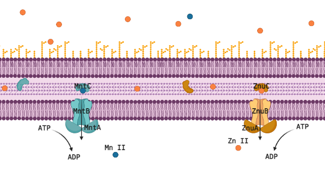
Many transition metals are critical cofactors for biological enzymatic reactions in animals like you and me, but also in bacteria. As cofactors, the properties of each metal ion are very unique, and one cannot be substituted for another, but they are all 2+ metal ions of similar size and weight, so proteins designed to transport or sequester these valuable resources often have affinity for multiple metal ions. For pathogenic bacteria this is a liability that makes them especially vulnerable to their host manipulating the concentrations of these ions up or down to induce toxicity or starvation. The human immune system primarily manipulates Zn (II), critical in its own right, but also a competitor for Mn (II), which is a cofactor for reducing reactive oxygen species (ROS); too much Zn (II) will outcompete Mn (II) and the cell will succumb to oxidative stress. The ATP-Binding Cassette (ABC) transporters MntABC and ZnuABC are at the heart of this system and have both been proven critical for pathogenic bacteria to successfully withstand an immune response and cause infection. Understanding this metal ion system could let us eventually target and interfere with it, posing a very promising new class of antibiotic drugs.
The Zn (II) and Mn (II) transport systems are incredibly sensitive, suggesting a fast-acting regulatory system that can rapidly respond to changes in the environmental and internal concentrations of these ions and to the needs of the cell. Professor Shivani Ahuja’s structural biochemistry lab is well equipped to capture this regulatory interaction red handed, but the involved proteins must be identified and purified to do that. We wouldn’t know which proteins to purify though, the present literature just doesn’t have strong candidates for post translational regulation of metal ion ABC transporters. This is where computational methods offer the chance to use disparate data from multiple species to piece together regulatory mechanisms for MntABC and ZnuABC.
The Protein Interactome
Protein interactomes are network models (also called graphs) of the proteins in an organism and the interactions between them. Obviously, the word interactions is vague, and usefully so even: it can make just as much sense to show genetic regulation interactions, co-expression, cytogenetic closeness, sequence similarity, and other kinds of biologically relevant relationships besides what I’ll call “physical interactions,” but at the heart of protein interactomes are those physical interactions. A physical interaction refers to 2 proteins associating together as a complex or in an allosteric interaction; the gold standard for proving this kind of interaction is the protein pull-down assay. Protein interaction data in the STRING database is the cornerstone of our analysis. The first thing we set out to do was to recreate the single species protein interactome models in Python using data from STRING and to make a very human-legible and well integrated interface for the interactome on Graphspace. Below is an example of a Graphspace interactome alongside the protein information and linked databases available for every node.
STRING’s interaction data is broad in scope but it often comes from experiments that follow a “shotgun” approach favoring coverage over accuracy. There are false positives and missing interactions and lots of interactions that occur under under experimental conditions but not in a cell. These limitations are all of particular concern for less-studied proteins with uncorroborated interactions, bacterial ABC proteins and their neighbors fall in this group. One of the main conceits of this project was to create multi-species interactomes to get a more reliable look at the interactions of ABC transporters and hopefully to find promising regulatory proteins.
Assayed protein interactions are supposed to mimic the interactions inside a cell so the data is specific to each species. However, because the ABC metal ion transport system is well conserved in most bacteria and any one species is likely to have incomplete or unreliable data, we set out to match homologous proteins between species to cross-reference interactions. This proved easier said than done as naming conventions between species were rarely descriptive and had little relation to each other. Matching homologous proteins using their names and meta data had little success. Querying other databases, like UniProt, ran into the same problems of incomplete or incompatible names and annotations when comparing between species. The interactomes we were able to generate had poor homology coverage which made it infeasible to rank interactions algorithmically and searching them by hand didn’t produce any obvious promising results.
While this foray into multi-species interactomes didn’t yield compelling results for our research question, it was an exciting project with many takeaways for further research. Establishing homology between species will require more consistently rich data, like sequence data, and would likely benefit from the use of multiple methods including sequence alignments, ontology data, and annotated meta data. Also, while human legible models are very important for sanity checks and meaningfully interpreting the interactome with respect to a given research question, it can be a bit of a liability. In the course of this project the data and analyses included in the interactome were limited by what could be represented in the visualization when they didn’t have to be. Separating what was running “under the hood” from what was visualized with Graphspace would have allowed more freedom to include rigorous analyses. Factoring these considerations into future work promises a very useful tool for estimating protein-protein regulatory interactions in the ABC transport system and beyond!
Hi, my name is Henry Jacques (he/him). I’m a class of 2024 biochemistry/molecular biology major here at Reed, and I spent this summer working with Max Bennett to (try to) develop a method of visualizing protein-protein interactions related to a target protein in bacteria with a tool called Graphspace (http://graphspace.org/).
Goals Though a stated goal of ours was to develop a program that worked across many species of bacteria and with many target proteins, we focused on Mn- and Zn-transporting molecules called ATP binding cassette transporters (ABC transporters) in B. subtilis, E. coli, S. aureus, and S. lugdenesis. These proteins are understood to play a vital role in metal ion homeostasis across many bacterial species, many of which are pathogenic. This focus was done at the direction of both Anna Ritz and Dr. Shivani Ahuja in the Chemistry department, who has taken a keen interest in the function and structure of these proteins.
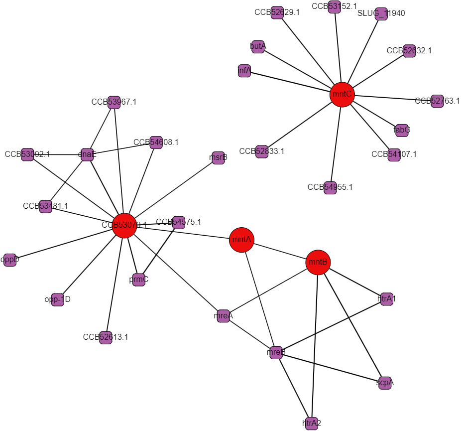
Methods We developed an algorithm to interpret data from individual bacterial species’ datasets on STRING, a database compiling protein-protein interaction data from research- and homology- based data sources. Data was taken as pairs of STRING identifiers signifying individual protein linkages and translated using a combined list of linkages between STRING identifiers and ‘common’ names for ease of interpretation in the final graph.
A secondary structure of these graphs was comparing the homologous interactions across species, which was done using homology data embedded in STRING as well as data from Clusters of Orthologous Groups (COG) mappings. These linkages were challenging to filter in terms of confidence, as STRING’s indication of homology leaves a lot to be desired in terms of ease of use. Nevertheless, we believe that the homologous interactions present could provide a useful starting point for future biochemical investigations using known homology data.
Challengesand next steps Perhaps the most cumbersome part of this project was reconciling the various naming conventions used for proteins across various interaction databases. STRING conventions were the primary identifiers used in internal recognition of protein-protein interactions, though many STRING identifiers were unmapped to more ‘common’ protein identifiers, thus making the data difficult to use for any biochemical interaction investigation without first translating the STRING identifiers.
Another challenge we encountered was that STRING’s dataset was mostly composed of non-experimental evidence, meaning that interactions inferred from such database were not necessarily supported by in vitro analysis in laboratory conditions. In some instances, interactions known to exists biochemically were not present as discrete data within the relevant STRING dataset, and had to be manually added for creation of the final graph. However, this lack of data presents one significant point at which even the incomplete data can be extrapolated for useful biochemical results: with further configuration of the graph generation, undiscovered interactions between known proteins with homologous known interactions in similar species can be hypothesized to exist, possibly providing a starting point for future biochemical research.
There’s certainly a lot more to be done with this project — whether it’s future me or someone else who tackles it, I hope it goes well 🙂
Hello world! My name is Nina Young (she/her) and I’m a junior Computer Science-Art major. This summer I had the amazing opportunity to work with Anna Ritz on the Signaling Pathway Reconstruction Analysis Streamliner (SPRAS) tool that she’s been developing in collaboration with some folks at UW-Madison.
A more in-depth overview of what signaling pathway reconstruction does is available here, but in essence we are creating networks made up of various proteins and connecting them based on how they are known to interact with each other. The hope is that by studying protein-protein interactions of interest, we can discover some intermediate proteins that are biologically significant and useful for further study. The SPRAS tool is useful because it consolidates a number of useful algorithms that approach network analysis in different ways, which will allow people who are less familiar with programming to make use of these algorithms quickly and efficiently.
So my job this summer was essentially to get familiar with the innards of SPRAS and ultimately implement a new algorithm into the program. All new contributors to the SPRAS project undergo an introductory tutorial in which they implement a simple algorithm, LocalNeighborhood, while familiarizing themself with how the program is organized. SPRAS is primarily written in Python, but it also makes use of SnakeMake and Docker to parallelize the program and keep all supplementary files in one place, respectively. The first part of the summer we worked through this introduction slowly, and I helped to refine the language of the tutorial and make it clearer for future contributors.
Once we had a handle on the tutorial and made some updates, I got to work implementing a simple algorithm called AllPairsShortestPaths. As the name suggests, this algorithm takes a network with source and target nodes as input and finds the shortest paths between all possible combinations of sources and targets. Though relatively simple, this algorithm will be a useful addition because it forms the framework for more complicated algorithms such as BowTieBuilder, which finds intermediate proteins that a number of paths cross.
Ultimately, this summer was a fascinating introduction to SPRAS, and I really admire what Anna and her team are doing in making this form of protein interaction analysis more accessible. I am hopeful that the work I did this summer helped strengthen the program’s foundation so that it can be easily expanded upon in the future.
Hi, my name is Alex Richter (she/her). I am a recent graduate from Reed College and post bac researcher with Anna Ritz. This is my second summer doing research with Anna Ritz. The project of this summer dealt with letters of recommendation and the role of gendered words/phrases.
The Problem
There are certain words and ways of describing people that appear in letters of recommendation that are gendered. These issues are implicit and occur regardless of the race, gender, or ethnicity of the writer. This issues leads to a disparity of women in specific fields due to the importance of letters of recommendation in graduate school acceptances and hiring.
A very easy example is that women are more likely to be praised in letters of recommendation for their communication or being nice. Men on the other hand are likely to be praised on their ability to do a task or a skill that is relevant to the position. It should also be noted that most of the research in this topic deals with a gender binary of just men and women. Our work tries to avoid the binary by focusing on pronouns, but it should be noted that in discussing this topic phrases such as “Male vs Female” or “Man vs Woman” are common place.
Why does it matter?
Letters of recommendation are important as they allow a better insight into a persons’ character. It is an important factor in hiring a candidate or accepting a candidate into any program. It shows more than just the accomplishments but speaks to who the individual is and how they are perceived by someone who knows them.
This work matters especially at Reed because of the emphasis we put on letters of recommendation. Notoriously, Reed does not give out grades unless requested and while transcripts with letter grades exist the letter grade concept is de-emphasized here. Reed focuses on quality and understanding as opposed to emphasizing grades. As stated in the letter that accompanies all transcripts, “Since its founding, Reed College has adhered to a distinctive educational philosophy, a critical component of which is the evaluation and grading of student academic work.”
Screenshot of PDF included with Reed transcripts to highlight grading policy
The Pre-Existing Work
In 2018, there was a project done by a graduate student named Mollie Marr and other collaborators. The repository for this project can be found here. This work entailed writing detectors that could be run in order to see if specific words were present in letters of recommendation. There were many detectors that were written by multiple developers. Each detector had been extensively researched and was backed by various publications.
The preexisting detectors that were implemented or suggested: – Female Detector / Male Detector: Identifies gendered female or male terms respectively. – Gendered Words Detector: Identifies whether the gender of the candidate is being brought to attention unnecessarily. – Personal Life Detector: Letters of recommendation for women are more likely to mention facts about their personal life. – Publication Detector: Letters of recommendation for women are less likely to mention publications and projects. – Effort (vs Accomplishment) Detector: This one is from a very impactful paper in this topic by Trix and Psenka. Women are more likely to be described using effort words while men are more likely to be described as accomplished or having an innate ability to do the task required. – Superlative Detector: Letters for women are less likely to contain superlatives. If they do, they usually describe women in the context of emotional terms. – Conditional Superlative Detector: This deals with superlatives that are “hedged” by restricting the population to only women.
The summer work for this project is dealing primarily with implementing more detectors and making this into an easily accessible resource for people. Future work would deal with creating a google docs or Microsoft word plug in or website. A major issue in this work has been dealing with the lack of a cohesive data set of letters of recommendation. This is due to the difficulty in anonymizing letters of recommendation.
Below is a list of citations that was included in the genderbias repository for any desired future inquiry into this problem.
Publications, Projects, and Research Trix, F. & Psenka, C., “Exploring the color of glass: Letters of recommendation for female and male medical faculty,” Discourse & Society 14(2003): 191-220.
Superlatives Dutt, K., Pfaff, D. L., Bernstein, A. F., Dillard, J. S., & Block, C. J. (2016). Gender differences in recommendation letters for postdoctoral fellowships in geoscience. Nature Geoscience, 9(11), 805.
Schmader, T., Whitehead, J., & Wysocki, V. H. (2007). A linguistic comparison of letters of recommendation for male and female chemistry and biochemistry job applicants. Sex Roles, 57(7-8), 509-514.
Nouns Trix, F. & Psenka, C., “Exploring the color of glass: Letters of recommendation for female and male medical faculty,” Discourse & Society 14(2003): 191-220.
Minimal Assurance Isaac, C., Chertoff, J., Lee, B., & Carnes, M. (2011). Do students’ and authors’ genders affect evaluations? A linguistic analysis of medical student performance evaluations. Academic Medicine, 86(1), 59.
Trix, F. & Psenka, C., “Exploring the color of glass: Letters of recommendation for female and male medical faculty,” Discourse & Society 14(2003): 191-220.
Effort Deaux, K. & Emswiller, T., “Explanations of successful performance on sex-linked tasks: What is skill for the male is luck for the female,” Journal of Personality and Social Psychology 29(1974): 80-85
Isaac, C., Chertoff, J., Lee, B., & Carnes, M. (2011). Do students’ and authors’ genders affect evaluations? A linguistic analysis of medical student performance evaluations. Academic Medicine, 86(1), 59.
Steinpreis, R., Anders, K.A., & Ritzke, D., “The impact of gender on the review of the curricula vitae of job applicants and tenure candidates: A national empirical study,” Sex Roles 41(1999): 509-528
Personal Life Isaac, C., Chertoff, J., Lee, B., & Carnes, M. (2011). Do students’ and authors’ genders affect evaluations? A linguistic analysis of medical student performance evaluations. Academic Medicine, 86(1), 59.
Madera, J. M., Hebl, M. R., & Martin, R. C. (2009). Gender and letters of recommendation for academia: Agentic and communal differences. Journal of Applied Psychology, 94(6), 1591.
Trix, F. & Psenka, C., “Exploring the color of glass: Letters of recommendation for female and male medical faculty,” Discourse & Society 14(2003): 191-220.
Gender Stereotypes Axelson RD, Solow CM, Ferguson KJ, Cohen MB. Assessing implicit gender bias in Medical Student Performance Evaluations. Eval Health Prof. 2010 Sep;33(3):365-85.
Foschi M. Double standards for competence: theory and research. Ann Rev Soc. 2000;26:21–42.
Gaucher, D., Friesen, J., & Kay, A. C. (2011, March 7). Evidence That Gendered Wording in Job Advertisements Exists and Sustains Gender Inequality. Journal of Personality and Social Psychology.
Hirshfield LE. ‘‘She’s not good with crying’’: the effect of gender expectations on graduate students’ assessments of their principal investigators. Gender Educ. 2014;26(6):601–617.
Madera, J. M., Hebl, M. R., & Martin, R. C. (2009). Gender and letters of recommendation for academia: Agentic and communal differences. Journal of Applied Psychology, 94(6), 1591.
Ross DA, Boatright D, Nunez-Smith M, Jordan A, Chekroud A, Moore EZ (2017) Differences in words used to describe racial and gender groups in Medical Student Performance Evaluations. PLoS ONE 12(8): e0181659.
Sprague J, Massoni K. Student evaluations and gendered expectations: what we can’t count can hurt us. Sex Roles. 2005;53(11):779–793.
Steinpreis RE, Anders KA, Ritzke D. The impact of gender on the review of the curricula vitae of job applicants and tenure candidates: a national empirical study. Sex Roles. 1999;41(7):509–528.
Trix, F. & Psenka, C., “Exploring the color of glass: Letters of recommendation for female and male medical faculty,” Discourse & Society 14(2003): 191-220.
Wenneras C, Wold A. Nepotism and sexism in peer review. Nature. 1997;387(6631):341–343.
Raise Doubt Trix, F. & Psenka, C., “Exploring the color of glass: Letters of recommendation for female and male medical faculty,” Discourse & Society 14(2003): 191-220.
Madera, J. M., Hebl, M. R., Dial, H., Martin, R., & Valian, V. (2019). Raising doubt in letters of recommendation for academia: gender differences and their impact. Journal of Business and Psychology, 34(3), 287-303.
ShorterLength of Letters Dutt, K., Pfaff, D. L., Bernstein, A. F., Dillard, J. S., & Block, C. J. (2016). Gender differences in recommendation letters for postdoctoral fellowships in geoscience. Nature Geoscience, 9(11), 805.
Trix, F. & Psenka, C., “Exploring the color of glass: Letters of recommendation for female and male medical faculty,” Discourse & Society 14(2003): 191-220.
Hi! I’m Lixing Yi, a rising sophomore, and this summer I have been implementing code to count directed graphlets and utilizing the data to categorize biological networks. Intending to be a math major, I have spent more of my time on the theoretical aspect of things. While I’ve learned about graphs and algorithms before, working on this project has been a refresher, as it’s a different way of interaction with these math concepts- to think about what the results means in a real-world context; to do a lot of trials and errors instead of “pure thinking”. It’s also an eye-opener for me to realize the vast opportunities in fields that I’ve not thought of before.
What are directed graphlets?
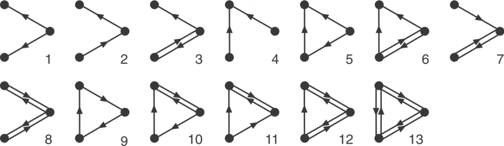
Graphlets are small, connected simple graphs. In our context, a graphlet is usually not alone an entire graph but an induced subgraph of a bigger graph. And namely, directed graphlets are graphlets with directed edges, like arrows between two nodes (vertices). For our context, we also allow bi-directional edges, which are edges that has arrows on both ends and can go both ways. We represent those edges by a pair of opposite-pointing edges.
Now we can define orbits. Node orbit are labels assigned to node positions in a graphlet. Intuitively, two nodes have the same orbit if they are symmetric. Rigorously, it means that permuting the two nodes with the same orbit will result in the exact same graphlet. Edge orbit follows the same idea, and it can be determined by node orbits: two edge have the same edge orbit if and only if the node orbits on their end nodes are the same.
That’s a brief introduction of graphlets! Hannah also explains the undirected version in her post. We are interested in them because the occurrence (or the lack of) these small graphs as induced subgraphs of a bigger graph might suggest interesting information of the big graph. On a node-level, the orbits that a node participates in can say things about the functionality of that node. Many biological networks are directed graphs, but due to the complexity of directed graphlets, our earlier work treats the edges as undirected. Thus, my work focuses on making tools to enable analysis with directed graphlets.
How do we count them?
Before discussing all the tricks to make the counting faster, let’s see the bottom line: There is always the brute force method. If we want to count all the four-node graphlets for example, we need to exhaust every connected four-node groups, and match this group with one of all 199 four-node graphlets. In comparison, there are only 6 undirected four-node graphlets. Each matching test is a mini graph isomorphism problem, so the run time adds up quickly, making the brute force method unideal.
To make the search more efficient, we use a method named GTrie, developed by Pedro Rebeiro et al. In short, it uses a decision tree to reduce the search space of graphlets we try to match. At every node, we start a BFS search to find all graphlets involved with it. Every time we discover a new node, we gain partial information about the potential graphlets and can eliminate some choices. For example, If the algorithm discovers a bi-directed edge during the search, then it will skip all graphlets without bi-directed edges at the final matching step. If it discover a triangle, then it will get rid of graphlets containing no triangles. When a graphlet is matched, the algorithm updates the graphlet and orbit counts. For a more detailed introduction, please refer to Rebeiro’s paper.
Another general approach to count directed graphlets is to count only certain graphlets, and then combinatorially build linear equations and compute the counts for the rest based on this information. This method is indeed faster than the Gtrie approach and is the one we use for undirected graphlet analysis. However, due to the complexity of directed graphlets, building linear equations becomes much more difficult and time-consuming that it outweighs the run time advantage. Another practical factor is that Gtrie already has code implementation while the linear equation approach only has a theoretical description. Behind the scenes, most of my time has been spent on configuring the Gtrie implementation to work.
Why do we count them?
Directed graphlet and orbit counting has many applications, but for our project we mainly used graphlet counting to characterize different biological networks. Beyond the number of nodes and edges, graphlet count provides substantially more dimensions for network comparison. In simple terms, we are now able to say “network A is different than network B in the sense that A has much fewer graphlet no. 5, but they both have similar number of graphlet no. 27.” However, we can’t just naively compare the graphlet counts of two networks directly, as the two networks might have very different sizes and inherently have very different graphlet counts. A direction of improvement would be to normalize the graphlet count by the number of nodes and edges. But how exactly? Since graphlets are very different than nodes or edges, we can’t just divide the grpahlet count by node count or edge count. For this task, we chose the Erdős–Rényi model, a random graph generating model. Given the count of a specific graphlet in a specific network, we calculate the probability1 and the confidence level that this count occurs in an Erdős–Rényi random graph with the same number of nodes and edges2.
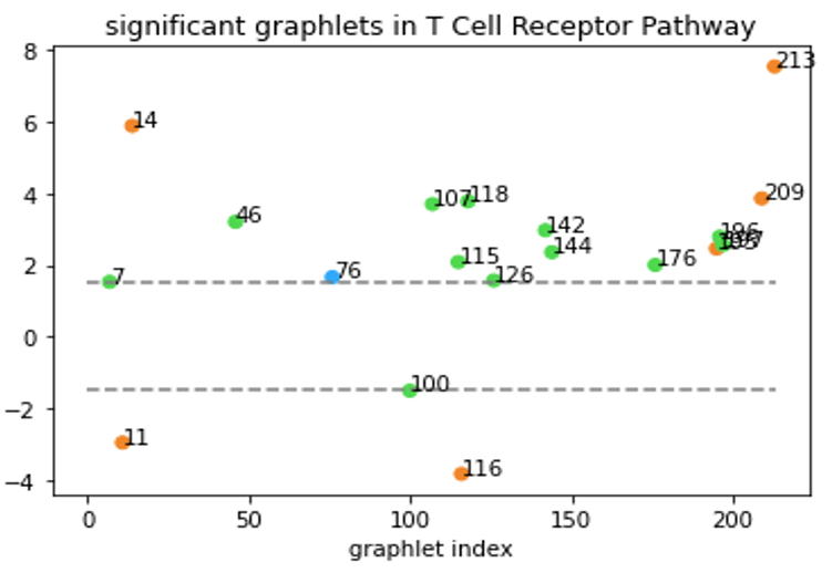
Although Erdős–Rényi model serves as a functioning null model for statistical comparison, it might still be “too random” and the confidence level based on this model might not reflect the real-world statistical significance. In a biological context, the more relevant question might be “how does this network compare to networks of similar type?” Clearly, that’s not an easy question. But to at least partially answer the question, we tentatively define “networks of similar type” as networks that have the same degree sequence. In our directed graph context, the notion of degree sequence is trickier with different types of edges, as discussed below3. To generate null-models under this restriction, we used the random-rewire algorithm. It randomly picks two edges (the stricter version would require them to be the same type), swaps the nodes on the edges, and repeats this process many times. This way, it randomizes the network while keeping the degree sequence the same, thus accomplishing our task of generating “networks of similar type”. We then generated 100 such graphs for a given specific network and computed the statistical significance of the graphlet counts for this network comparing to our null model. An example of our results is shown below.
Graphlets with z-score >1.5 or < -1.5 are shown. All-bidirectional graphlets are orange, all-one-directional are blue. Graphlets with both bidirectional and one-directional edges are green.
Now, we are able to say “T Cell Receptor Pathway has a lot of graphlet no. 213” without causing any confusions!
Future work
You might have noticed that I didn’t mention orbits in my work. For the time being, I only get to work on the general graphlet count, but I’m excited to see what new insights we will gain by incorporating node/edge orbits into the analysis. What’s more, we will also incorporate directed graphlet counting with Hannah’s project on MCL clustering for community detection. Some of the networks that Hannah worked on are directed networks, and we are hoping a directed clustering algorithm will bring more accurate results. The clustering algorithm will also require an edge orbit count which the Gtrie software doesn’t do yet, but it’s a fun challenge to devise an algorithm for this task.
Reference
[1] Pedro Ribeiro, Fernando Silva. G-Tries: an efficient data structure for discovering network motifs. https://www.dcc.fc.up.pt/~pribeiro/pubs/pdf/ribeiro-acmsac2010.pdf [2] The Gtrie implementation that I modified: https://www.dcc.fc.up.pt/got-wave/
Thanks for reading all the way to the end! Here’s the footnotes.
The probability of an induced subgraph in a Erdős–Rényi graph is discussed here. It’s one of those things that everyone agrees it’s true but no one bothers to give a rigorous proof. (laugh)
Erdős–Rényi graph generation with a specified edge count: I came up with this algorithm using random shuffle: for a n node graph, create all n2 edges, then do a Fisher-Yates random shuffle. Then just chop off the first k edges, k being the number of edges specified. This algorithm takes O(n2) time, which I don’t think can be further improved.
In my implementation, only the total degree sequence was kept the same, the in-degree, out-degree, and bi-degree sequence were randomized. Whether this would make sense in our biological context, I’m honestly not sure. The more conservative and strict rule would be to keep the degree sequence of each type of edges the same. But then, I worry such restrictions would be too strict that the randomization won’t accomplish much. For the best results, we would do both methods and see how the results differ.
Hi! My name is Hannah Kuder, I’m a rising math-physics senior working in Anna Ritz’s lab this summer. My project has focused on implementing a graphlet-based version of the Markov Clustering (MCL) algorithm on various biological interactomes in order to compare those clusterings to normal MCL. In particular, whether any of the graphlets cluster disease genes “better”.
Graphlets
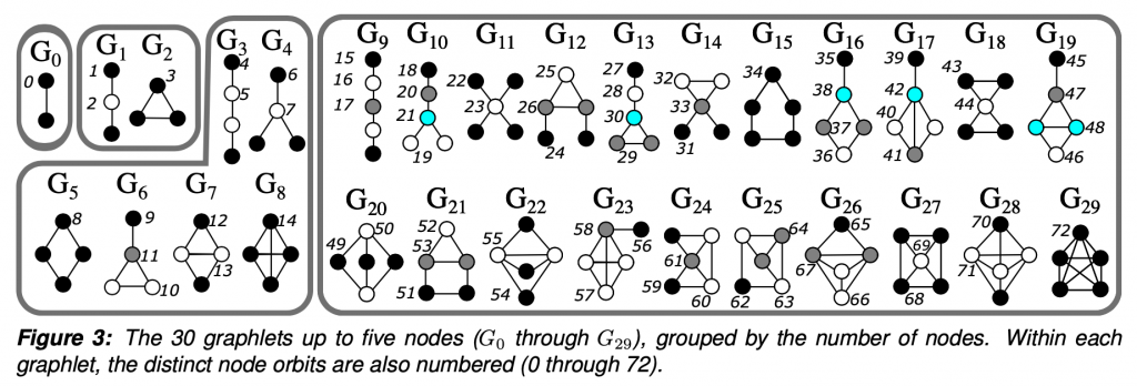
To put it simply, graphlets are connected induced subgraphs. Starting at G0, we have all of the connected induced subgraphs that can be created from 2 nodes, which is just an edge. I focused this project on graphlets up to 5 nodes.
Taken from Anna and Pramesh’s graphlet grant proposal.
The “induced” part of the definition means that given a subgraph that looks exactly like G29, a 5 node clique, we would not say that G15, the 5 node ring is also present. Given 5 connected nodes, there is only one 5 node graphlet present. The graphlet must contain all of the edges between the selected nodes.
So why graphlets? They are a way to investigate patterns and the higher order structure of the network. In between the very local level of two nodes being connected by an edge, which doesn’t tell us about any greater trends, but much less global than a statistic such as density, which misses much of the network-specific intricacies.
Markov Clustering
Markov Clustering essentially simulates a random walk. Given an edge list, MCL creates a transition matrix, where every column and row represent a node with the entry [i,j] being the probability a transition from one node to the other could occur. MCL then cycles between two steps: expansion and inflation.
Expansion simulates a normal random walk (taking the power of the probability matrix using the normal matrix product)
Inflation accentuates high probabilities and diminishes lower probabilities (taking the power entrywise aka the Hadamard power)
In the implementation of MCL, there is a parameter you can choose called the “inflation parameter” which controls how far those probabilities are exaggerated. A lower inflation parameter means less “inflation” and thus a coarser clustering and larger clusters, while a higher inflation parameter produces more, smaller clusters. Which inflation parameter to use is dependent on both the specific network and your goals.
With each cycle of inflation and expansion, clusters are found. Taken from the official MCL website, https://micans.org/mcl/index.html.
Graphlet-Based MCL
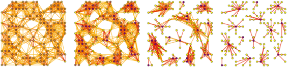
So the main idea behind this project is to combine the two and see if any graphlet-based versions of MCL uncover anything insightful that normal MCL could not. To combine the two, for a given graphlet, all of the edges that did not participate in the given graphlet were deleted. MCL then performed clustering on the graph that remained. Thus we are left with 30 different clusterings of the same network.
Specifically, I have been focusing on a protein-protein interactome (ppi) with 21,559 proteins and 342,353 edges. This interactome contains genes associated with 519 diseases. Each of the 30 different versions of MCL produced different clusterings of these genes. I am currently trying to compare the results of the different higher-order graphlets to G0, which is normal MCL.
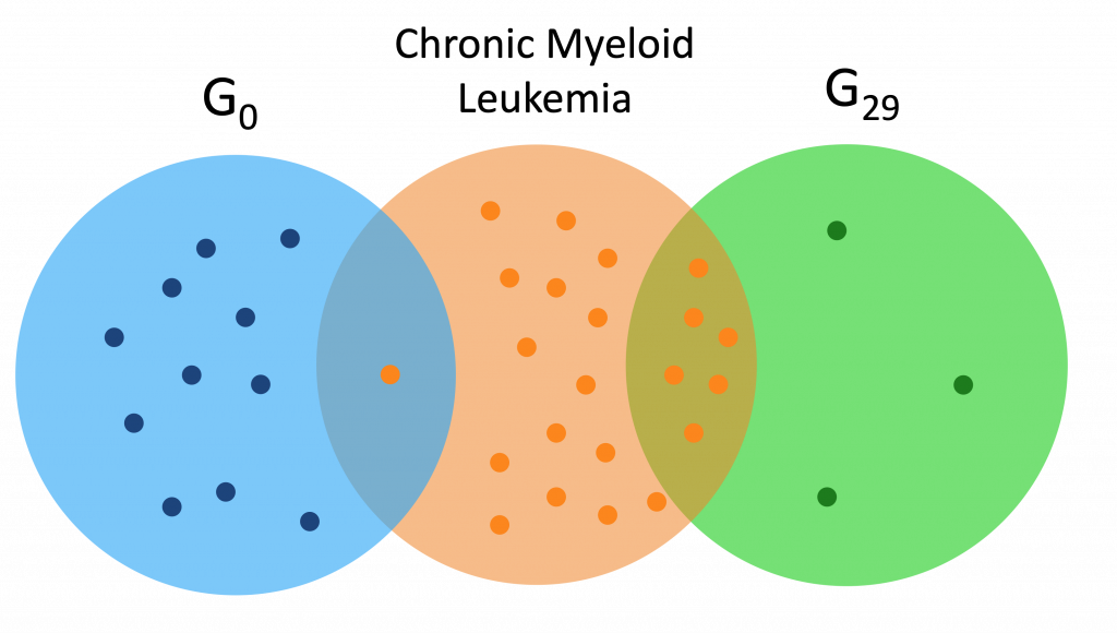
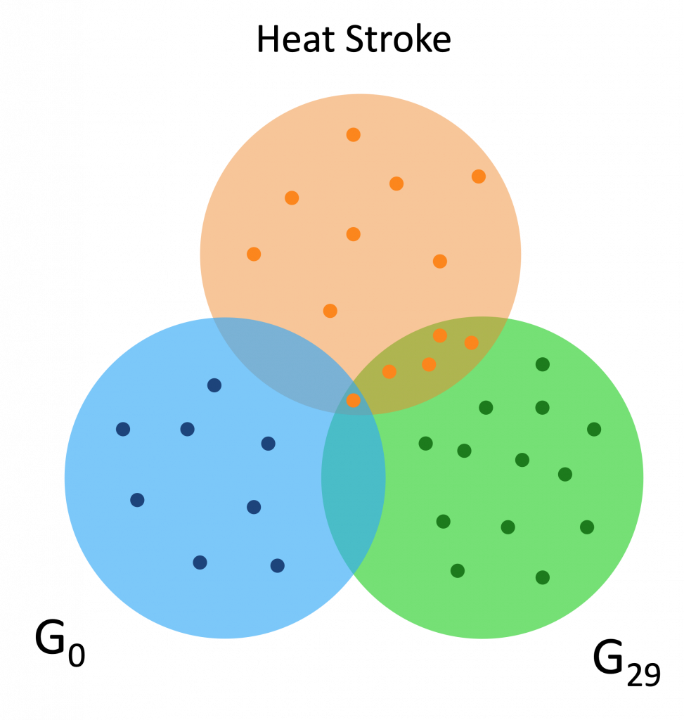
Here are a couple Venn diagrams comparing the “best” clusters from G0 and G29 for a couple diseases. “Best” means the cluster had the most disease genes in it.
Each of the dots is a gene, while the orange dots are disease genes.
We see that in these diseases, the best cluster of G29 is much more enriched than the best cluster of G0.
I have also calculated the hypergeometric score for each of these best clusters across all of the diseases, which is the probability that given N disease genes in a pool of M total genes, that a cluster with m genes would contain n disease genes. Essentially, is the number of disease genes in that cluster significant? Or is it likely to happen just by chance.
A problem I am facing with these hypergeometric scores is how to compare the probabilities across different graphlets, and hopefully I’ll figure something out before my research ends next week.
This summer is jam-packed with new research ideas and projects! Since the last posts in 2020, postdoctoral researcher Pramesh Singh has joined the group. We have also started some exciting collaborations with folks at UW-Madison, Tufts, and University of Florida. Here’s what we are up to for the next few weeks:
Streamlining pathway reconstruction algorithms with SPRAS. We are excited to continue working with Tony Gitter at UW-Madison to build SPRAS, a workflow to easily run multiple pathway reconstruction algorithms on multiple datasets. Nina Young is helping on this project as we add more downstream analysis functionality and incorporate new algorithms into the workflow.
Using networks to understand metal ion transport and homeostasis in bacteria. In this brand-new collaboration with Reed chemist Shivani Ahuja, Max Bennett and Henry Jacques are using network-based mapping, visualization, and analysis to identify conserved interactions that may be involved in regulating the ATP-binding cassette (ABC) transporter family, which are highly conserved in bacteria.
Studying the topology of disease genes using graphlets. Last year, we published a paper showing that using small, connected, induced subgraphs called graphlets to describe signaling pathways can compare these pathways across databases. Lixing Yi, Hannah Kuder, and Larry Zeng are working on related projects to implement a directed graphlet library, identify graphlet-enriched communities, and better understand graphlet-based measurements in networks. Pramesh is the research co-mentor on this project.
Tools to identify gendered language in student letters of recommendation. In a non-compbio project, post-baccalaureate Alex Richter is investigating existing methods to identify gendered language in evaluations, with a goal to build a tool to help faculty remove bias from their letters of recommendations. This project is funded by Reed’s Social Justice Research and Education Fund.
Stay tuned to hear more about these and other projects!
Hey everyone! I am Maham Zia and this summer I worked as a post-bacc for Anna Ritz (primary advisor) and Derek Applewhite (co-advisor). I graduated from Reed in May 2020 with a degree in Physics, but during my undergraduate career I worked in a cell biology and cellular biophysics lab. I am interested in how physics interacts with other disciplines such as biology and chemistry. I believe that interdisciplinary research transcends boundaries and aids the scientific community to think about a variety of problems in creative ways. This summer I put my coding skills to use by working on a computational project that involved analyzing images of cells. For her senior thesis, Madelyn O’ Kelley-Bangsberg ’19 used the punctate/diffuse index to measure the distribution of phosphorylated NMII Sqh. Punctate/diffuse index is widely used to measure the spread of fluorescently tagged cytochrome c in cells during apoptosis. Measuring this index involves determining standard deviation of the average brightness of the pixels using time lapse microscopy [1]. O’Kelley-Bangsberg’19 used the same idea to determine whether the cell has punctate phosphorylated myosin (high pixel intensity standard deviation) or diffuse phosphorylated myosin (low pixel intensity standard deviation). She did this in ImageJ by outlining each cell, obtaining an X-Y plot of the intensity and finally calculating the relative standard deviation ((standard deviation/mean pixel intensity) x 100 ) by setting the highest intensity value to 1 and lowest intensity value to 0. She used relative standard deviation instead of the absolute standard deviation to draw comparisons because she observed that mean pixel intensity values changed drastically between treatments [1]. Under Anna’s guidance I worked on automating this process in MATLAB by making use of image processing techniques which made the entire process a lot more time efficient.
I was working with images that each had two channels: (1) An actin channel that shows the distribution of actin- a double helical polymer that aids in cell locomotion and gives the cell its shape. Since actin is distributed throughout the cell, staining it allows us to see the entire cell [2]. (2) A channel showing the distribution of phosphorylated NMII Sqh.
The general idea was to use the actin image to detect/outline the cells and somehow use that information to plot the cell outline on the second image which has the distribution of the phosphorylated NMII Sqh. Plotting them would allow me to obtain the intensity values of the pixels within each cell and determine the standard deviation of the pixel intensity values for each cell.
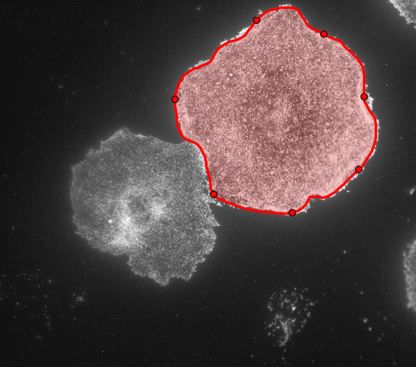
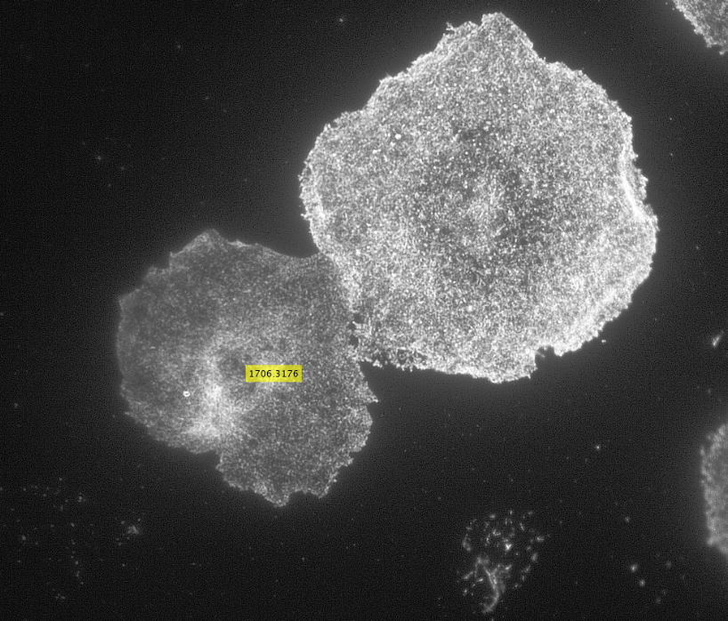
Initially, my code read in the image with the actin staining and used the inbuilt imfindcircles function in MATLAB to detect cells in the actin image. One of the input arguments of the function is radiusRange which can be used to detect circles with radii within a certain range. However, the function doesn’t work well for ranges bigger than approximately 50 pixels which means it doesn’t work well for images with both small and large cells. Moreover, the function has an internal sensitivity threshold used for detecting the cells. Sensitivity (number between 0 and 1) can be modified by putting it in as an optional argument when calling the function, but increasing it too much can lead to false detections [3]. Using imfindcircles function is not a robust way to detect cells and therefore I decided to switch to the drawfreehand function in MATLAB 2020 that allows the user to interactively create a region of interest (ROI) object.
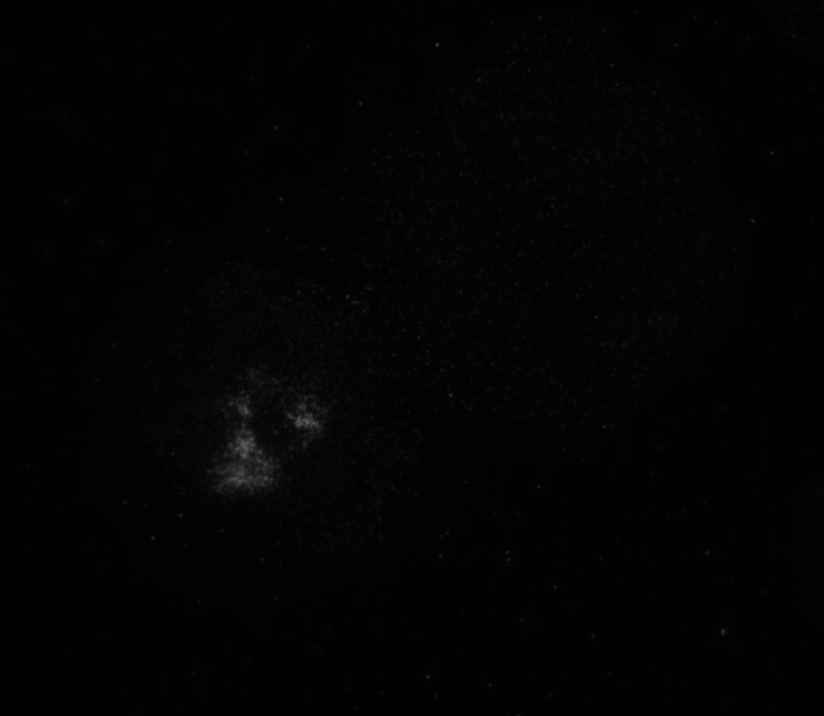
After creating the ROI object (in simple terms that means outlining the cell) as shown in the figure above, I created a binary mask and used regionprops to get the centroid and the equivalent diameter of the object. The code then read in the second image as shown below with the distribution of the phosphorylated NMII Sqh and used outputs from regionprops and the impixel function to get the pixel intensity values for each cell. This image mostly looks dark because it is only showing the distribution of phosphorylated NMII Sqh which is the small cluster of bright pixels we see.
Impixel function takes the column and row indices of the pixels to be sampled and gives their pixel intensity values. However, lengths of column and row vectors need to be the same and since I was approximating the cells as circles, the only way to extract the intensity values of the pixels was to think of a circle as enclosed in a square. So, I used the center coordinates and radii of the circles to get coordinates of the top left corner of the square and used the linspace function to get equally spaced vectors for column and row. Finally, std2 and insertText functions were used for calculating the standard deviation values and displaying them on the image showing the actin distribution respectively.
Future goals could involve analyzing a number of images to determine reasonable standard deviation values and finding a way to extract pixel intensity values for pixels only within the ROI object instead of a square enclosing the object to calculate standard deviation values.
Now that I am done with this project, for this upcoming year I will be working as a research assistant in a lab part of the department of Genetics, Cell Biology, and Development at the University of Minnesota.
References:
[1] M. O’Kelley-Bangsberg, Reed undergraduate thesis (2019) [2] J. Wilson and T. Hunt, Molecular Biology of the Cell: The Problems Book (Gar- land Science, New York, NY, 2008), 5th ed., ISBN 978-0-8153-4110-9, oCLC: 254255562. [3] MathWorks, “Detect and Measure Circular Objects in an Image”, https://www.mathworks.com/help/images/detect-and-measure-circular-objects-in-an-image.html