Computing network statistics on the GIANT network turned out to be somewhat of a challenge! The first hurdle that Alex and I discovered is that the brain-specific network we are working with is enormous, containing around 43 million edges. This network size was simply too big to run any program on efficiently, so Anna stepped in and created a file of “trimmed” networks that we could quickly use for our computations. Essentially, the edges in the network are weighted by a certain probability, so the network was trimmed by choosing a probability threshold; edges with weights less than that probability would not be included in the trimmed network. The largest trimmed network had about 6.4 million edges and a probability threshold of 0.125. I ran my statistics on networks with probability thresholds of 0.150, 0.175, 0.200, and 0.300 to see if there were differences in the statistics and what those differences might reveal about the structure of the network.
The statistics I ran on the trimmed networks were degree distribution, average AND, and shortest path length distribution. The degree distribution is the most straightforward – the degree of a node in a graph is the number of nodes it is connected to, so the degree distribution is a a histogram of the number of nodes in the network with a certain degree. The shape of the curve provides information about the structure of the graph. If you take the log of the degree distribution, a nice downward sloping line tells you that the network is scale-free, meaning its degree distribution follows what is known as the “power law distribution.” Scale free networks generally contain a smaller number of nodes with a high degree and a higher number of nodes with a small degree.
Below is the degree distribution for the trimmed network with a probability threshold of 0.150. All degree distributions calculated on the trimmed networks looked the same.

AND is short for the average neighbor degree – this looks at a node and sees how many neighbors (nodes a node is connected to) its neighbors have. Average AND answers the following question: On average, what is the degree of the neighbors of nodes with a certain degree? This question essentially investigates if there is a pattern in the degree of neighbors of nodes with a certain degree. Once again, the slope of the line reveals a piece of information about the structure of the network. A negative correlation means high degree nodes tend to be connected to low degree nodes, also known as a disassortative network. A positive correlation means high degree nodes tend to be connected to other high degree nodes and low degree nodes tend to be other low degree nodes, also known as an assortative network. The following figure from a paper on biological network connectivity demonstrates this concept quite clearly:

Overall, the average AND plots of the trimmed networks appear to be assortative, though the shape differs slightly. For example, compare the average AND plots of trimmed networks with 0.150 (top), 0.175 (middle), and 0.300 (bottom) threshold probabilities:


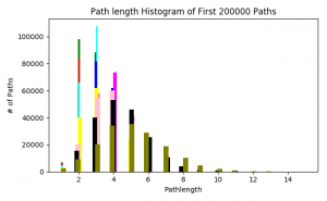
The final statistic is the path length distribution. This statistic is calculated using the breadth-first search algorithm to determine the length of shortest paths between all nodes. However, due to the size of the networks, my program doesn’t look at all possible paths between all nodes, instead running the BFS algorithm twice; once until it hits 100,000 paths and again with 200,000 paths. This was mainly done to see if there was a huge difference in the distribution of path lengths. There is a slight difference, as demonstrated by the distributions of the trimmed network with 0.150 probability threshold:


The next step for this statistic is to normalize the number of paths and see what difference this makes. Over the next couple of weeks, my goal is to refine my positive set of genes and check the GIANT brain-specific network to see if any of these genes appear.


