Category: Uncategorized

This week, I ran some statistics on how our existing SZ gene dataset fit within the GIANT network. I found that most of our genes had a posterior probability of about 0.3-0.5. Which makes sense, given that many of our genes should be at least 0.2.

Next/this week is thanksgiving, but soon we’ll be setting parameters for how we want to judge each gene in the completed network given the qualities of the GIANT network as a whole.

Computing network statistics on the GIANT network turned out to be somewhat of a challenge! The first hurdle that Alex and I discovered is that the brain-specific network we are working with is enormous, containing around 43 million edges. This network size was simply too big to run any program on efficiently, so Anna stepped in and created a file of “trimmed” networks that we could quickly use for our computations. Essentially, the edges in the network are weighted by a certain probability, so the network was trimmed by choosing a probability threshold; edges with weights less than that probability would not be included in the trimmed network. The largest trimmed network had about 6.4 million edges and a probability threshold of 0.125. I ran my statistics on networks with probability thresholds of 0.150, 0.175, 0.200, and 0.300 to see if there were differences in the statistics and what those differences might reveal about the structure of the network.

The statistics I ran on the trimmed networks were degree distribution, average AND, and shortest path length distribution. The degree distribution is the most straightforward – the degree of a node in a graph is the number of nodes it is connected to, so the degree distribution is a a histogram of the number of nodes in the network with a certain degree. The shape of the curve provides information about the structure of the graph. If you take the log of the degree distribution, a nice downward sloping line tells you that the network is scale-free, meaning its degree distribution follows what is known as the “power law distribution.” Scale free networks generally contain a smaller number of nodes with a high degree and a higher number of nodes with a small degree.

Below is the degree distribution for the trimmed network with a probability threshold of 0.150. All degree distributions calculated on the trimmed networks looked the same.

AND is short for the average neighbor degree – this looks at a node and sees how many neighbors (nodes a node is connected to) its neighbors have. Average AND answers the following question: On average, what is the degree of the neighbors of nodes with a certain degree? This question essentially investigates if there is a pattern in the degree of neighbors of nodes with a certain degree. Once again, the slope of the line reveals a piece of information about the structure of the network. A negative correlation means high degree nodes tend to be connected to low degree nodes, also known as a disassortative network. A positive correlation means high degree nodes tend to be connected to other high degree nodes and low degree nodes tend to be other low degree nodes, also known as an assortative network. The following figure from a paper on biological network connectivity demonstrates this concept quite clearly:

Overall, the average AND plots of the trimmed networks appear to be assortative, though the shape differs slightly. For example, compare the average AND plots of trimmed networks with 0.150 (top), 0.175 (middle), and 0.300 (bottom) threshold probabilities:

The final statistic is the path length distribution. This statistic is calculated using the breadth-first search algorithm to determine the length of shortest paths between all nodes. However, due to the size of the networks, my program doesn’t look at all possible paths between all nodes, instead running the BFS algorithm twice; once until it hits 100,000 paths and again with 200,000 paths. This was mainly done to see if there was a huge difference in the distribution of path lengths. There is a slight difference, as demonstrated by the distributions of the trimmed network with 0.150 probability threshold:

The next step for this statistic is to normalize the number of paths and see what difference this makes. Over the next couple of weeks, my goal is to refine my positive set of genes and check the GIANT brain-specific network to see if any of these genes appear.

 

This week, I got more familiar with the NetworkX package, which is concerned with graph based programming. It’s very powerful, but the complete GIANT network is far too large for it to run efficiently. Even the 0.1 threshold for edges has 41 million edges. However, Anna showed that the number of edges decreases exponentially as the threshold goes up. A careful balance will be needed as for the weight we put on these edges in our final program and how many we include.

This week, I compared the brain tissue specific network from human base (http://hb.flatironinstitute.org) with the set of genes I collected associated with a higher risk of schizophrenia. This tissue specific network gives the probability that 2 genes interact with each other specifically in the brain. Genes that interact in regions other than the brain but still interact in the brain have a lower probability count. As expected, nearly all of the associated genes had at least a 0.1 probability, which is relatively high in terms of bioinformatic confidence. Notably, several of the genes interactions that had above a 0.9 probability involved cell adhesion genes.

Of the genes below the 0.1 confidence, most do have neural roles but simply have roles common to other parts of the body. For instance, mir-137 is involved in neural development but is also involved in tumor suppression for several cancers.

This upcoming week, I will be learning how to use NetworkX and will be gathering statistics from the Humanbase network with it.

This past week, I created a unified standard for genes. Now regardless of the naming preferences for the genes that various research databases provide, I can now manipulate them as if they were all following the same naming conventions. This resulted in about 10 new genes being added to the gene overlap sets from all the different collections of genes.

This week, I am going to compare all of these genes to that of the GIANT network. That way, we can know where these genes specifically are and what processes they are involved in.

I am also going to be hunting for negatives to compare against for when we build the more complex program. Genes completely uninvolved in Schizophrenia are actually really difficult to find, given that all of the genes I hold in this collection are about 8% of the protein coding genome. I’ll look at computational biology papers associated with mental disorders similar to Schizophrenia, like autism.

Fall break is over and we’re back to work!

Before break, I found a great resource that summarizes cell motility proteins by grouping them by function; it includes chemotaxis, receptors, growth factors, rho family GTPases, adhesion, integrin-mediated signaling, cellular projections, cell polarity, and proteolysis. This resource constitutes a significant portion of the positive set of proteins involved in cell motility.

Over the past week, I have entered the next step in creating my positive set of proteins known to be participants in cell motility and schizophrenia. Because many papers cited pathways (in addition to specific proteins), it’s crucial to look at these pathways and comb proteins from them to add to the positive set. These pathways, which include the CAM pathway, FAK pathway, and Reelin pathway, were taken from KEGG, a pathway database. Unfortunately, the KEGG pathways download as unreadable XML files, so I must parse these files; I am currently using a parser developed by Anna Ritz. After I have parsed these pathways, my next small step is to see which, if any, proteins are involved in multiple pathways.

Once my positive set has come together, I will begin analyzing the GIANT network. This includes comparing KEGG proteins to the GIANT network as well as generating summary statistics of the GIANT network. I will go into more detail of what this entails as I complete this portion of my analysis, but it will include generating statistics such as degree distribution, average node degree (AND), average AND, and possibly a few others.

The week before break, at the group meeting, we discussed the gene lists Miriam and I created. Because of the lack of overlap on my part, my next job to do is to modify my program to account for possible different gene names. Anna sent me a giant text file for it, and I will get it done by the Friday meeting.
I did not spend all of break dormant, and I learned more about bayesian statistics in addition to a brief overview by one of Anna’s post-docs. I think one of the difficulties of knowing how Bayes’ theorem works is the fact that it’s just so ingrained into our normal thought. Given B, what is the probability of A? It’s the probability of B given A times the probability of A divided by the probability of B. The first thing to note is the B denominating the whole equation. The B is accounting for the probability warping from the context of the problem. The second factor is probability of B given A. This represents the relationship we already know. This is multiplied by the probability of A. Therefore, the numerator represents the total probability of B happening because of A, which can also be described as the total probability that the specified relationship happens. By accounting for the probability warping in the denominator, we get the actual probability of A given B.
Bayesian probability is the core of the functional interaction network and the integrated network we will make. I can already kind of see how gene interaction probabilities could be derived from this given interaction data.
However, the mutual exclusivity clause in the theorem might be tricky. I’ll have to closely look at the supplemental data to see how the functional interactive builders accounted for this.

Currently on break. Will resume blog posts next week.

This week, Anna drafted me to make a program to find the common genes in my schizophrenia dataset. It was a little tricky, given that all of the datasets from the different studies were organized differently, but it wasn’t anything I couldn’t handle.

Legend:

108 LOCI

Schizophrenia Working Group of the Psychiatric Genomics Consortium (2014). Biological insights from 108 schizophrenia-associated genetic loci. Nature 511, 421–427.
SZGENE

Allen, N.C., Bagade, S., McQueen, M.B., Ioannidis, J.P.A., Kavvoura, F.K., Khoury, M.J., Tanzi, R.E., and Bertram, L. (2008). Systematic meta-analyses and field synopsis of genetic association studies in schizophrenia: the SzGene database. Nat Genet 40, 827–834.
HIPSC

Brennand, K.J., Simone, A., Jou, J., Gelboin-Burkhart, C., Tran, N., Sangar, S., Li, Y., Mu, Y., Chen, G., Yu, D., et al. (2011). Modelling schizophrenia using human induced pluripotent stem cells. Nature 473, 221–225.
DEADEXPRESSION

Fromer, M., Roussos, P., Sieberts, S.K., Johnson, J.S., Kavanagh, D.H., Perumal, T.M., Ruderfer, D.M., Oh, E.C., Topol, A., Shah, H.R., et al. (2016). Gene expression elucidates functional impact of polygenic risk for schizophrenia. Nat Neurosci 19, 1442–1453.
CHROMOSOME CONFORMATION

Won, H., de la Torre-Ubieta, L., Stein, J.L., Parikshak, N.N., Huang, J., Opland, C.K., Gandal, M.J., Sutton, G.J., Hormozdiari, F., Lu, D., et al. (2016). Chromosome conformation elucidates regulatory relationships in developing human brain. Nature 538, 523–527.

 

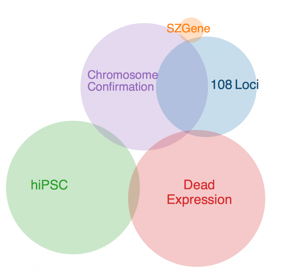
The first thing to note is that there was one gene that was in every data set except SZGene that couldn’t be included in this diagram because the Venn diagram program I found online deemed it geometrically impossible. This gene is TCF4, also known as immunoglobulin transcription factor 2. It is implicated in Pitt-Hopkins Syndrome and is involved in initiating neural differentiation.

An overlap between hiPSC, DeadExpression, and Chromosome Conformation is PRICKLE2, or Prickle Planar Cell Polarity Protein 2. It seems to be involved in the growth of post synaptic densities and neurite outgrowth.

Another pertinent overlap is EFHD1. EFHD1 was found in 108 Loci, hiPSC, and Chromosome Conformation. It seems to be calcium dependent and involved in apoptosis and neural differentiation, and it’s probably mitochondria dependent. However, its family is involved in cytoskeletal rearrangement.

One possibility for the dearth in overlap is simply the diversity in methods. Each collection got its genes from different areas, and it’s very likely that gene expression is totally different in all of these contexts. I’ll probably ask Anna more about this later. Until then, I will restart my Bayesian studies.

Over the past couple of weeks, Alex and I have been given the task of building our project’s gold standard list. This list will be comprised of genes known to be associated with Schizophrenia and genes known to be associated with cell motility; Alex was given the Schizophrenia half to research and I was given the cell motility half. Overwhelmed by the sheer volume of genes and pathways associated with cell motility, I began by looking up genes known to be associated with both Schizophrenia and cell motility. In our meeting, we briefly discussed how this might serve us later as a known positive we could use to test our algorithm.

I read through tons of articles and papers, many of which I found through references in previous papers we have read. In reading these papers, I was hunting for genes, pathways, and resources that were studied and employed by the researchers and found several that will be useful to us. The CAM pathway and associated genes appeared multiple times, and the resource KEGG was used by the majority of the researchers. My task over the past week has been to download data from KEGG, continue accumulating genes for our gold standard list, and begin adding “confidence details” to the genes – this is an important weight that will be added to the genes in our list and will be a measure of how “confident” we are that the gene is truly associated with either Schizophrenia or cell motility.