The Pathway Not Taken – Page 6 – Computational Biology Research at Reed College

Bayesian Weighting Schemes

Week 2 Progress Report

Week 2 was spent further looking into Bayesian Weighting Schemes and in particular how they were applied in a specific paper titled Top-Down Network Analysis to Drive Bottom-Up Modeling of Physiological Processes by Poirel et. al. This was the original LINKER paper that PATHLINKER was built upon. I also spent a very decent amount of time looking at other interactomes and curating a working list of interactomes and how they weight their interactomes. So far I have only done this in detail for the HIPPIE interactome but more work is still needed. Besides research, I also worked on a document about Bayesian Weighting that aims to elucidate some of the mathematical set up and notation for the paper mentioned above as it suffered from some convoluted mathematical notation. Hopefully, this will be useful to people trying to read this paper in the future. Other tasks involved debugging code, presenting learned material and sorting through papers to find relevant papers.

Summer Week 1: Prime Nodes

This week, I got caught up with the state of the project. Anna and Miriam had cleaned up and optimized our code to the point where it could be submitted and run in a reasonable amount of time. However, there still remained the problem of nodes only connected to positives. Since positives are held at a constant score of 1.0, and negatives at a constant 0.0, any nodes only connected to a positive will have a score of 1.0, which misrepresents how a gene fits within the polygenic nature of schizophrenia and cell motility.

To solve this, we decided to make three networks, each one identical to the one we were previously testing. However, there are two key differences.

The positives are divided between the three networks.
The three nodes in each networks representing their gene are also connected to a prime node that is only connected to those three nodes. The prime node’s score is the node by which we judge a gene.

This reduces the edge cases where a gene is only connected to a positive or a negative, since the gene cannot be connected to only one node. This also allows us to evaluate positive nodes within the context of all other positives. If a positive node is found to be positive in other networks, then the score will be high. Even the neighbor positives within the same network will diffuse the positivity through their prime nodes down to other networks, increasing the score for the neighbor of the positive and therefore increasing the score for the positive.

One thing to note is that the AUC seems to be relatively stable despite the network threshold or the prime node implementation. However, my guess is that this is probably due to the positives generally being only vaguely functionally related. Also, only 116 SZ genes are in the 0.200 network, reducing the polygenic power of our method. One thing to try is to add more genes from other studies. I will research other studies to find more gene lists and p-values.

Yen’s k shortest paths

This week, we split up to delve further into the PathLinker paper according to our aims. I was assigned to research Yen’s k-shortest paths algorithm and present to the lab on Wednesday.

I’m now going to attempt to explain this algorithm–bear with me.

Some caveats: first, this is an algorithm for computing the k-shortest loopless paths from one node to another, and this algorithm only considers simple paths, where nodes may not be repeated.

To compute the k-shortest paths (where k is a user-defined parameter, say 10 or 4), we first find the shortest path (k=1) using some sort of algorithm, say Dijkstra’s.

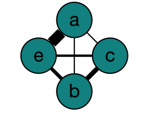
Here’s our wonderful graph from Graphspace:

Start Node	End Node	Weight
a	b	1
a	c	1
a	e	9
b	e	3
b	c	4
c	e	2

So, using our graph, let’s find the shortest path from a to e (P_1). Looking at the graph, we can see that it is a->c->e, with cost 4. Now what we do is loop through all paths using this first path as a guide, because intuitively, there might be some obvious edges that we use in many of the shortest paths.

Let’s call what we’re using from P_1 the root path, and call what we use when we diverge from it the spur path. To find P_2 (the 2nd shortest path), we must go through the graph differently this time to make sure we just don’t get the shortest path again. Because we’re using P_1 as a guide, let’s pretend that the edge from a->c has infinite cost, so that we can never take that edge.

The paths that result from the root path being (a) is then [a ->b->e (4), a->e(9), a->b->c->e(7)].

Then, we expand our root path to be a->c, and pretend that the edge c->e has infinite cost, so the next path is [a->c->b->e (8)].

We combine the two lists of potential paths and look at their costs. [a->b->e (4), a->e(9),a->b->c->e(7), a->c->b->e(8)]. a->b->e is the 2nd shortest path (P_2)!

Then, we can simply search through the rest of the list for the next shortest path (P_3,…,P_k).

Week 2: Understanding Wnt/β-catenin Signaling and the Ryk-CFTR-Dab2 Path

This week, Kathy, Usman, and I split up to learn more about different aspects of PathLinker. I researched the Wnt/β-catenin signaling pathway, precision-recall curves, and the role of CFTR and Dab2. On Wednesday, we all presented the topics we had researched to each other and Anna and Ibrahim.

To briefly summarize what I learned, the Wnt/β-catenin pathway regulates the transcription of certain genes related to cell proliferation, cell attachment, and growth. When the Wnt/β-catenin signaling pathway is dysregulated, a number of pathologies can develop including cancer and heart disease. In fact, in a study on colon adenocarcinoma by the Cancer Genome Atlas, 93% of tested tumors had a mutation that affected the Wnt/β-catenin signaling pathway (TCGA, 2012). At the most basic level theWnt/β-catenin signaling pathway is turned on when Wnt proteins bind to “frizzled” a 7-pass transmembrane receptor which halts the destruction of β-catenin in the cell. Usually, when the pathway is off, β-catenin is constantly being produced and destroyed. When β-catenin destruction is interrupted, β-catenin will build up in the cytoplasm and move into the nucleus where it will bind to LEF and the TCF promoter to promote the transcription of specific genes that were previously being inhibited by a transcription factor that was bound to TCF. The Wnt/β-catenin signaling pathway involves many proteins and interactions, some of which we still do not understand. The PathLinker algorithm succesfully identified a path in the Wnt/β-catenin signaling pathway that was not in the KEGG or NetPath database: the Ryk-CFTR-Dab2 path (Ritz et al, 2016). The authors of the paper hypothesized that Ryk would interact with CFTR (Cystic Fibrosis Transmembrane-conductance Regulator), a chlorine ion channel previously studied for its role in cystic fibrosis, which would activate Dab2 to inhibit β-catenin activity. This hypothesis was experimentally confirmed by silencing Ryk, CFTR and Dab2 individually using RNA interference and then testing transcription levels of β-catenin controlled genes using a TCF/LEF luciferase activity and levels of β-catenin in the cell using a Western Blot assay.

We also attended a data management workshop taught by David Isaak, Reed’s data science librarian to learn how to use Git and GitHub. Because I’ve never really used terminal before (I usually use repl.it), I worked through a command line tutorial to learn more about it.

On Thursday, Kathy, Usman, and I went through our Dijkstra code with Anna, and finally got it to work the way we wanted it to. Anna added us to the cancer-linker repository on GitHub so we can all begin to actually work on PathLinker now.

My next project is to figure out how to take data from FireBrowse, a database containing data from TCGA on 38 different cancer types, put it into a format we can use, and apply several statistical analyses to the information. I’m hoping to base it off of PepperPathway, a program written by Nicholas Egan, a student in Anna’s lab last summer, that uses data from FireBrowse, GeneCards and NetPath and to create a visual representation on GraphSpace. I’m struggling to make sense of the PepperPathway program because there are a lot of files on the GitHub repository and I’m not really sure where to begin. I’m going to try to make sense of it this weekend.

References

TCGA Research Network. Comprehensive Molecular Characterization of Human Colon and Rectal Tumors. July 19, 2012. Nature. DOI: 10.1038/nature11252.
Ritz, Anna et al. “Pathways on Demand: Automated Reconstruction of Human Signaling Networks.” Npj Systems Biology And Applications 2 (2016): 16002. Web.

Week 1

Aim of Research Project

My research project aims to extend upon the original PATHLINKER paper. In particular, I hope to investigate different weighting schemes both from the perspective of utilizing different data sets and data-summary methods as well as potentially maybe different statistical tools for manipulating the data in meaningful ways. This is motivated by the fact that there appears to be little overlap between interactomes consisting of the same proteins but weighted differently. Therefore, this project will allow us to analyze different schemes and develop an heuristic for weighting interactomes. As a result, we will be able to apply algorithms like PATHFINDER on graphs such that they provide results that have valid biological meaning rather than being affected by superficial factors such as trends in scientific research or biases of the scientific community. Right now, I am focusing on Bayesian Weighting schemes which attempt to use experimental evidence to provide a weight that represent the probability of a given interaction occurring in a given signaling pathway by leveraging Bayes’ theorem. I will talk more about this in future posts.

Week 1 Progress

Week 1 was spent mostly acquainting myself with the necessary prerequisite knowledge required for research during coming weeks such as Dijkstra’s algorithm (and its implementation) and Bayesian Weighting Schemes and in that regard reading some relevant papers. For the sake of keeping track the particular papers were titled :-

The first was the original PATH LINKER paper which our research hopes to extend upon. The next two provided some information on Bayesian Weighting but did not provide too much else due to some ambiguous mathematical notation. I hope to attempt to write a document that annotates the relevant portions of the papers for the sake of clarity and future reference.

Week 1

Sol, Usman, and I have started working on summer research to modify the PathLinker algorithm.

This week, we plan to finish the code implementing Dijkstra’s algorithm on toy datasets, which was used as a warmup exercise in order to acclimatize us back into working and coding. In addition, I’ve been assigned to understand Yen’s k-shortest paths algorithm, which is one of the foundations of PathLinker.

Week 1

This is Kathy, Usman, and my first week working on our summer research projects which all involve modifying the PathLinker algorithm. For my project, I am interested in integrating data about protein methylations related to colon adenocarcinoma from the FireBrowse database into PathLinker. Protein methylation, which is only one of many ways that cell signaling pathways can be altered in cancerous cells, can either inhibit or enhance protein-protein interactions. I intend to devise a way to use this information to change the weights of edges connected to methylated proteins to more accurately model cancerous cell signaling pathways. I am hoping this method could eventually be generalized so that the algorithm could be modified for multiple types of cancerous mutations. I believe that this work could be important in identifying important proteins for further research.

So far, we have mostly been trying to learn about pathway reconstruction methods before we dive in. To do this, we have been re-reading the original PathLinker paper as well as a more recent paper about an alteration to PathLinker that allows it to integrate protein localization information.

We have also been working on understanding and implementing two algorithms that calculate the shortest path from a source to a target in a graph: Breadth First Search and Dijkstra’s algorithm. Breadth-first search is an algorithm that finds the path with the fewest number of edges from a source to a target. Dijkstra is more advanced and relative to our work because it takes the weight of the edges between nodes into account. Dijkstra will find the path with the lowest sum of edge weights from the source to any node in the graph.

This weekend and this coming week I have several goals. Primarily, Usman, Kathy and I need to figure out how to get the separate pieces of code that we wrote for the Dijkstra algorithm (which all work individually) to work together to first read a text file, then run Dijkstra’s algorithm, and finally produce a visual graph that shows the best paths. I need to do more research about the original PathLinker to gain a better understanding of precision-recall curves which were used to evaluate its efficacy, Ryk-CFTR-Dab2, which is a new path that was discovered in the Wnt/β-catenin signaling pathway by PathLinker, and the experimental methods that were used to verify the importance of CFTR.

Week 23

I ran the bulk-BLASTer to find good homology targets from our results

Derek Applewhite, our cell biology advisor, noted that several top genes could be novel to flies, and several genes could be novel to cell motility.

Miriam and I will continue to work out the bugs in the verification system for our process.

Week 23

This week, my goals have been relatively simple and short. There are a couple of bugs in my code that I need to sort out. I haven’t been able to collect any data about how “good” our method is due to these bugs, but once I do, we will hopefully be able to see that the results we are getting are not random.

Week 22

Since the last time I wrote a blog post, I have mainly been working on one way of verifying our algorithm; essentially, we need to make sure that our method is actually good at doing what it’s supposed to be doing. Although there are several ways to verify an algorithm, some of which Alex has been working on, I am working on something called “k-fold cross validation.”

This method of verification works by removing (or “hiding”) 1/k-th of your positives, then running your method and seeing where the hidden positives are ranked. You randomly choose the 1/k positives to hide and do this several times. You can also use the distribution of scores you get from each run to see how your method (with all positives) compares – are you getting significant results or are you getting what is expected from randomly choosing positives?

My first attempt at this was just a test run, and there were a few mistakes that I made. First, I chose to sample half instead of choosing a more reasonable number of positives such as 1/4 or 1/5. I also didn’t randomly choose positives to hide – I simply deleted the second half of the positives, and in doing so, might have removed an entire cell motility pathway or two from the positives. This would have produced biased results.

This coming week, my goal is to randomly sample 1/4 of positives multiple times, as well as implement some plotting functions in order to visualize the distribution of scores.