Hey everyone! I am Maham Zia and this summer I worked as a post-bacc for Anna Ritz (primary advisor) and Derek Applewhite (co-advisor). I graduated from Reed in May 2020 with a degree in Physics, but during my undergraduate career I worked in a cell biology and cellular biophysics lab. I am interested in how physics interacts with other disciplines such as biology and chemistry. I believe that interdisciplinary research transcends boundaries and aids the scientific community to think about a variety of problems in creative ways.
This summer I put my coding skills to use by working on a computational project that involved analyzing images of cells. For her senior thesis, Madelyn O’ Kelley-Bangsberg ’19 used the punctate/diffuse index to measure the distribution of phosphorylated NMII Sqh. Punctate/diffuse index is widely used to measure the spread of fluorescently tagged cytochrome c in cells during apoptosis. Measuring this index involves determining standard deviation of the average brightness of the pixels using time lapse microscopy [1]. O’Kelley-Bangsberg’19 used the same idea to determine whether the cell has punctate phosphorylated myosin (high pixel intensity standard deviation) or diffuse phosphorylated myosin (low pixel intensity standard deviation). She did this in ImageJ by outlining each cell, obtaining an X-Y plot of the intensity and finally calculating the relative standard deviation ((standard deviation/mean pixel intensity) x 100 ) by setting the highest intensity value to 1 and lowest intensity value to 0. She used relative standard deviation instead of the absolute standard deviation to draw comparisons because she observed that mean pixel intensity values changed drastically between treatments [1]. Under Anna’s guidance I worked on automating this process in MATLAB by making use of image processing techniques which made the entire process a lot more time efficient.
I was working with images that each had two channels:
(1) An actin channel that shows the distribution of actin- a double helical polymer that aids in cell locomotion and gives the cell its shape. Since actin is distributed throughout the cell, staining it allows us to see the entire cell [2].
(2) A channel showing the distribution of phosphorylated NMII Sqh.
The general idea was to use the actin image to detect/outline the cells and somehow use that information to plot the cell outline on the second image which has the distribution of the phosphorylated NMII Sqh. Plotting them would allow me to obtain the intensity values of the pixels within each cell and determine the standard deviation of the pixel intensity values for each cell.
Initially, my code read in the image with the actin staining and used the inbuilt imfindcircles function in MATLAB to detect cells in the actin image. One of the input arguments of the function is radiusRange which can be used to detect circles with radii within a certain range. However, the function doesn’t work well for ranges bigger than approximately 50 pixels which means it doesn’t work well for images with both small and large cells. Moreover, the function has an internal sensitivity threshold used for detecting the cells. Sensitivity (number between 0 and 1) can be modified by putting it in as an optional argument when calling the function, but increasing it too much can lead to false detections [3]. Using imfindcircles function is not a robust way to detect cells and therefore I decided to switch to the drawfreehand function in MATLAB 2020 that allows the user to interactively create a region of interest (ROI) object.
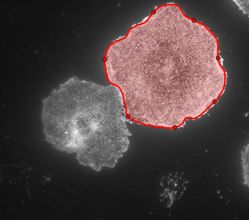
After creating the ROI object (in simple terms that means outlining the cell) as shown in the figure above, I created a binary mask and used regionprops to get the centroid and the equivalent diameter of the object.
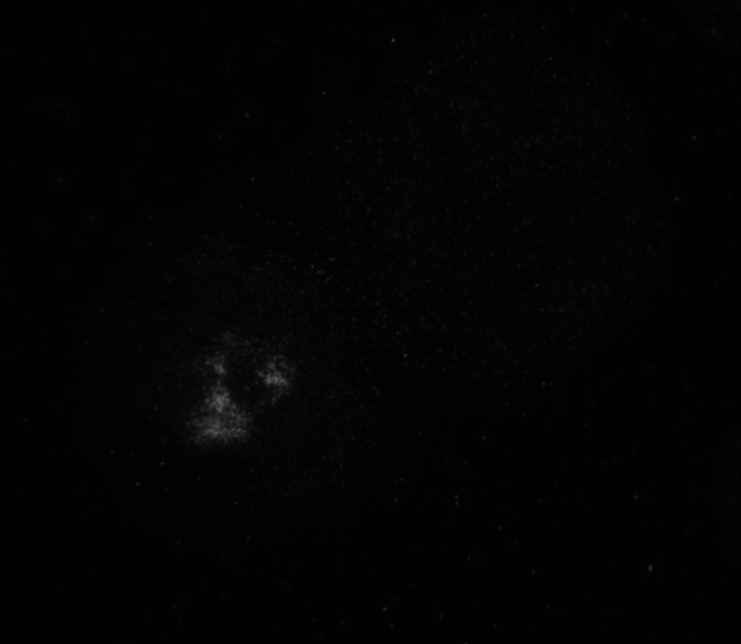
The code then read in the second image as shown below with the distribution of the phosphorylated NMII Sqh and used outputs from regionprops and the impixel function to get the pixel intensity values for each cell. This image mostly looks dark because it is only showing the distribution of phosphorylated NMII Sqh which is the small cluster of bright pixels we see.
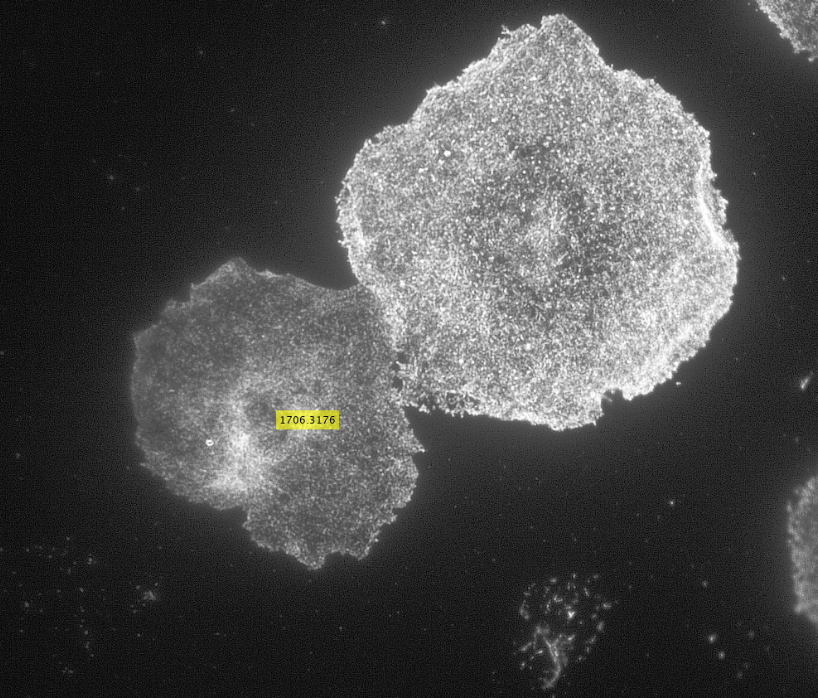
Impixel function takes the column and row indices of the pixels to be sampled and gives their pixel intensity values. However, lengths of column and row vectors need to be the same and since I was approximating the cells as circles, the only way to extract the intensity values of the pixels was to think of a circle as enclosed in a square. So, I used the center coordinates and radii of the circles to get coordinates of the top left corner of the square and used the linspace function to get equally spaced vectors for column and row. Finally, std2 and insertText functions were used for calculating the standard deviation values and displaying them on the image showing the actin distribution respectively.
Future goals could involve analyzing a number of images to determine reasonable standard deviation values and finding a way to extract pixel intensity values for pixels only within the ROI object instead of a square enclosing the object to calculate standard deviation values.
Now that I am done with this project, for this upcoming year I will be working as a research assistant in a lab part of the department of Genetics, Cell Biology, and Development at the University of Minnesota.
References:
[1] M. O’Kelley-Bangsberg, Reed undergraduate thesis (2019) [2] J. Wilson and T. Hunt, Molecular Biology of the Cell: The Problems Book (Gar- land Science, New York, NY, 2008), 5th ed., ISBN 978-0-8153-4110-9, oCLC: 254255562.
[3] MathWorks, “Detect and Measure Circular Objects in an Image”, https://www.mathworks.com/help/images/detect-and-measure-circular-objects-in-an-image.html